Numerical Solution of Eulerian Advection Equation in 1-D Operator Splitting

The Eulerian advection equation is solved numerically in 1-D by operator splitting over the x, y, and z directions. The process involves finite differencing of derivatives and ensuring conservation in steady and convergent flows. Different finite-difference approximations of derivatives are discussed, along with various numerical advection schemes like Forward Euler, Leapfrog, and Linear upstream schemes. The application of finite-volume upstream schemes helps in mass conservation and reducing interpolation errors. The concept of numerical diffusion in finite-volume upstream schemes is also explored.

Download Presentation

Please find below an Image/Link to download the presentation.
The content on the website is provided AS IS for your information and personal use only. It may not be sold, licensed, or shared on other websites without obtaining consent from the author.If you encounter any issues during the download, it is possible that the publisher has removed the file from their server.
You are allowed to download the files provided on this website for personal or commercial use, subject to the condition that they are used lawfully. All files are the property of their respective owners.
The content on the website is provided AS IS for your information and personal use only. It may not be sold, licensed, or shared on other websites without obtaining consent from the author.
E N D
Presentation Transcript
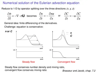
Numerical solution of the Eulerian advection equation Reduce to 1-D by operator splitting over the three directions (x, y, z): = n t nu x n t C t C x = = n U becomes u or General idea: finite differencing of the derivatives. Challenge: equation is conservative: n or C n C Steady flow Convergent flow Steady flow conserves number density and mixing ratio, convergent flow conserves mixing ratio Brasseur and Jacob, chap. 7.2
Finite-difference approximation of derivative d/dx Obtained by truncation of Taylor series; truncated term defines the order of approximation j value for gridpoint j j-1 j j+1 x xj-1 xj x xj+1 Taylor series: i i ( ) x d dx = + + 1 j j i ! i = 1 i j (x) d /dx . xj 1 xj xj+1 Brasseur and Jacob, chap. 4.8.1
First-order forward: d dx d dx ( ) ( ) 2 2 + 1 j j = + + = + ( ) ( ) x O x O x Taylor series: + 1 j j x j j Second-order central: ( ) 2 x 2 d dx d dx ( ) 3 = + + + ( ) x O x Taylor series (forward): + 1 j j 2 2 j j ( ) 2 x 2 d dx d dx ( ) 3 = + + ( ) x O x Taylor series (backward): 1 j j 2 2 j j d dx ( ) 3 = + 2 ( ) x O x Take difference: + 1 1 j j j d dx ( ) 3 + 1 2 1 j j = + ( ) O x x j
Numerical advection schemes can be diffusive and/or dispersive Advection of square wave in steady flow for 40 steps with Courant number = u t/ x = 0.5 C Forward Euler Forward Euler scheme: forward 1st-order derivatives in time and space Numerically unstable C t=40 Leapfrog Leapfrog scheme: central 1st-order derivatives in time and space Highly dispersive, negative values t=0 Exact C Linear upstream scheme: forward 1st-order derivative in time, 1st-order upstream derivative in space Upstream Highly diffusive Brasseur and Jacob, chap. 7.3.4
Finite-volume upstream schemes gridbox n n + = , , i t t i t ( ) ( ) un un 1/2, 1/2, + i t i t t Mass conservation is ensured; Interpolation error at gridbox edges is reduced by solving for momentum and scalars on staggered grids (C-grid): ui-1/2 ui+1/2 ni Brasseur and Jacob, chap. 7.4
Numerical diffusion in a finite-volume upstream scheme = u t/ x is the Courant number 1 n = 0.5 to xixi+1 xi+2 xi+3 n = 0.5 0.5 0.5 to + t xixi+1 xi+2 xi+3 1 true solution n 0.5 to + 2 t 0.25 0.25 xixi+1 xi+2 xi+3 Brasseur and Jacob, chap. 7.4
Numerical diffusion in a finite-volume upstream scheme with conservation of first-order moments (slopes scheme) 1 n = 0.5 to xixi+1 xi+2 xi+3 n 1 = 0.5 to + t xixi+1 xi+2 xi+3 1 true solution n 0.75 to + 2 t 0.25 0.25 xixi+1 xi+2 xi+3 Piecewise parabolic method (PPM) used in GEOS-Chem resolves subgrid distribution with a quadratic function to reduce numerical diffusion Brasseur and Jacob, chap. 4.8
Difficulty of preserving free tropospheric layers in Eulerian models = C t C u / 2-D pure advection of inert Asian plume in GEOS-Chem Advection scheme is 3rd-order piecewise parabolic method (PPM) Decay of plume maximum uniform flow Initial plume 2.5 days convergent/ divergent flow atmospheric flow 6 days 9 days Advection equation should conserve mixing ratio 3rd-order advection scheme fails in divergent/shear flow Increasing resolution yields only marginal improvement Rastigejev et al. [2010]
Why this difficulty? Numerical diffusion as plume shears A high-order advection scheme decays to 1st-order when it cannot resolve gradients (plume width ~ grid scale) Wind t = 0 t = h t = 2h Increasing grid resolution only delays the effect in sheared/divergent flow Wind shear t = 0 t = h t = 2h
Further investigation with 0.25ox0.3125o version of GEOS-Chem 2-D model grid at 0.25ox0.3125o, initial plume is 12ox15o 192 h Color measures volume mixing ratio (VMR) 96 h 144 h 0 h 48 h maximum mixing ratio Cmax Decay rate constant Cmax(t+h) = Cmax(h) exp[- h] Eastham and Jacob [2018]
Semi-Lagrangian advection Determine concentration at gridpoint (or grid vertex) A at time tn+1 = tn+ t by advecting a Lagrangian air parcel back in time over t and inferring the concentration at the departure point D by interpolation on the model grid Model grid Allows transport time steps larger than the Courant limit Single transport calculation for all species But does not conserve mass (posterior correction needed) Brasseur and Jacob, chap. 7.8
1. We talked about explosive vs. non-explosive behavior of chemical systems. Consider this simple 3-reaction mechanism where (1) chemical X is catalytically oxidized by the OH radical, producing chemical Y; (2) chemical Y photolyzes to produce OH; (3) OH is lost to particles. 1. X + OH Y + OH 2. Y + hv OH + 3. OH Assuming steady state for Y, show from the kinetic equations that this mechanism will either consume X explosively or will shut itself down, depending on the initial concentration of X. Kinetic equations: d[X]/dt = -k1[X][OH] k1[X][OH] = k2[Y] (steady state for Y) d[OH]/dt = k2[Y] k3[OH] So d[OH]/dt = k1[X][OH] k3[OH] = (k1[X]-k3)[OH] No steady state is possible for OH except if [X]=k3/k1 If [X] > k3/k1, d[OH]/dt > 0 and reaction is explosive; If [X] < k3/k1, d[OH]/dt < 0 and reaction shuts itself down.
2. We saw that the advection equation conserves mixing ratio, therefore a pollution plume should not dilute as it is transported in the atmosphere. But we know from personal experience that this is not true in the real world plumes in fact dilute. What is missing in this picture? Wind shear and stretch causes the plumes to split and stretch into mm-size filaments at which point molecular diffusion takes over molecular diffusion Wind du/dy>0 (shear) molecular diffusion Wind du/dx>0 (stretch) time scale for molecular diffusion: t = ( x)2/2D Molecular diffusion coefficient D ~0.1 cm2 s-1; x ~ 1 mm t ~ 0.1 s