Nyquist Stability Analysis in Control Systems
Explore Nyquist stability analysis in control systems, covering Nyquist theorem, path, plot, and examples. Learn about system stability, Nyquist criteria, avoiding singular points, and practical applications using Scilab. Enhance your knowledge of frequency response analysis in automatic control systems.
Download Presentation

Please find below an Image/Link to download the presentation.
The content on the website is provided AS IS for your information and personal use only. It may not be sold, licensed, or shared on other websites without obtaining consent from the author. If you encounter any issues during the download, it is possible that the publisher has removed the file from their server.
You are allowed to download the files provided on this website for personal or commercial use, subject to the condition that they are used lawfully. All files are the property of their respective owners.
The content on the website is provided AS IS for your information and personal use only. It may not be sold, licensed, or shared on other websites without obtaining consent from the author.
E N D
Presentation Transcript
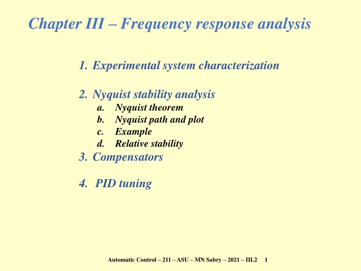
Chapter III Frequency response analysis 1. Experimental system characterization 2. Nyquist stability analysis a. Nyquist theorem b. Nyquist path and plot c. Example d. Relative stability 3. Compensators 4. PID tuning Automatic Control 211 ASU MN Sabry 2021 III.2 1
Open and closed loop poles System with unity feedback: Denominator of closed loop TF is: F(s) = 1 + G(s) Stability? Look for poles (i.e., roots of F(s) = 0) Y U G + U Y = ; G(s) + 1 G F(s)-domain s-domain Im Im F(s1) s1 pc Re Re pc: closed loop pole po: open loop pole po N.B.1: One-to-one correspondence If and only if F(s) analytic Automatic Control 211 ASU MN Sabry 2021 III.2 2
Nyquist theorem N = Nc No F(s)-domain s-domain Im Im Re Re Nc: number of enclosed closed loop poles No: number of enclosed open loop poles N: number of encirclement of origin N > 0 if clockwise; N <0 if anticlockwise Automatic Control 211 ASU MN Sabry 2021 III.2 3
Nyquist path & Nyquist plot G(j )-domain s-domain Im Im ( , ) Re 1 + j0 Re Nyquist path Nyquist plot [G(j ) = F(j ) 1] Also called polar plot G(s) = const NB1: On the lims Need to consider only s = j N.B.2: if G(j ) = passes by 1+j0 Marginally stable Automatic Control 211 ASU MN Sabry 2021 III.2 4
Avoiding singular points in Nyquist path Example: G = K/(s j 0) /2 G = Ke j / N.B.3: Singular point: pole or zero of G(j ) On s j 0 = ej , = /2 G(j )-domain s-domain Im Im Re Re Automatic Control 211 ASU MN Sabry 2021 III.2 5
Nyquist example 1 + 6 20 s s N = Nc No ( ) = G s ( )( ) + 2 4 s No = 1 N = 1 Nc = 0 Stable Plotted using Scilab: s = poly(0,'s'); G = (6*s+20)/((s 2)*(s+4)) sl = syslin('c',G); nyquist(sl); Automatic Control 211 ASU MN Sabry 2021 III.2 6
Nyquist example 2 N = Nc No 3 9 1 + s ( ) = G s ( )( ) + 3 s s No = 0 N = 2 Nc = 2 Unstable Plotted using Scilab: s = poly(0,'s'); G = (3 9*s)/((s+1)*(s+3)) sl = syslin('c',G); nyquist(sl); Automatic Control 211 ASU MN Sabry 2021 III.2 7
Stability margins Gain margin km Phase margin m 20 Log |G| Positive Gain margin km Im 1 / km Log 1 + j0 Re m Log Positive Phase margin m G Automatic Control 211 ASU MN Sabry 2021 III.2 8
Remark: relative stability Relative Stability = real parts of all poles: i < | To check relative stability using Nyquist: (same as we did for Routh) Put: s = s' | Apply Nyquist on G(s') Automatic Control 211 ASU MN Sabry 2021 III.2 9


