Optical Fiber Waveguides: Ray Theory Transmission and Refraction

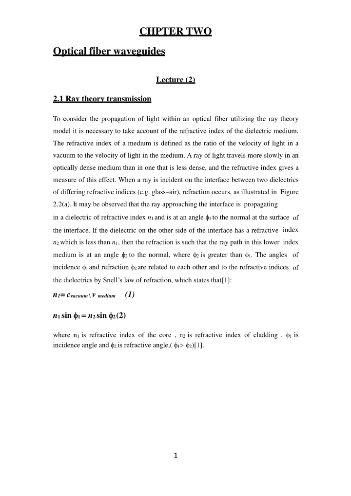
CHPTER TWO Optical fiber waveguides Lecture (2) 2.1 Ray theory transmission To consider the propagation of light within an optical fiber utilizing the ray theory model it is necessary to take account of the refractive index of the dielectric medium. The refractive index of a medium is defined as the ratio of the velocity of light in a vacuum to the velocity of light in the medium. A ray of light travels more slowly in an optically dense medium than in one that is less dense, and the refractive index gives a measure of this effect. When a ray is incident on the interface between two dielectrics of differing refractive indices (e.g. glass air), refraction occurs, as illustrated in Figure 2.2(a). It may be observed that the ray approaching the interface is propagating in a dielectric of refractive index n1and is at an angle 1to the normal at the surface of the interface. If the dielectric on the other side of the interface has a refractive index n2which is less than n1, then the refraction is such that the ray path in this lower index medium is at an angle 2to the normal, where 2is greater than 1. The angles of incidence 1and refraction 2are related to each other and to the refractive indices of the dielectrics by Snell s law of refraction, which states that[1]: n1= cvacuum \v medium (1) n1 sin 1 = = n2 sin 2(2) where n1 is refractive index of the core , n2 is refractive index of cladding , 1 is incidence angle and 2is refractive angle,( 1 2)[1]. 1

It may also be observed in Figure 2.2(a) that a small amount of light is reflected back into the originating dielectric medium (partial internal reflection). As n1is greater than n2, the angle of refraction is always greater than the angle of incidence. Thus when the angle of refraction is 90 and the refracted ray emerges parallel to the interface between the dielectrics, the angle of incidence must be less than 90 . This is the limiting case of refraction and the angle of incidence is now known as the critical angle c, as shown in Figure 2.2(b). From Eq. (1) the value of the critical angle is given by[1]: sin c = n2\ n1 (3) Total Internal Reflection(TIR): It occurs at the interface between two dielectrics of differing refractive indices when light is incident on the dielectric of lower index from the dielectric of higher index, and the angle of incidence of the ray exceeds the critical value (i.e. incidence criticalandn1 n2) see fig(2c)[1]. 2

Meridional Ray: The ray which passes through the axis of the fiber core[1], see Fig. (2.3). Acceptance angle( ( a): It is the maximum angle to the axis at which light may enter the fiber in order to be propagated, and is often referred to as the acceptance angle* for the fiber. see fig. (2.4)[1]. Numerical aperture: It is possible to continue the ray theory analysis to obtain a relationship between the acceptance angle and the refractive indices of the three media involved, namely the core, cladding and air. This leads to the definition of a more generally used term, the numerical aperture of the fiber. see fig.(2.5)[1]. 3

The ray enters the fiber from a medium (air) of refractive index no, and the fiber core has a refractive index n1, which is slightly greater than the cladding refractive index n2. Assuming the entrance face at the fiber core to be normal to the axis, then considering the refraction at the air core interface and sing Snell s law given by Eq. (2)[1]: nosin 1= n1sin 2 (4) Considering the right-angled triangle ABC indicated in Figure 2.5, then: =?- 2 ? where is greater than the critical angle at the core cladding interface. Hence Eq. (4) becomes: no sin 1 = n1cos Using the trigonometrically relationship sin2 + cos2 = 1, Eq. (2.5) may be written in the form: = c & 1 = a then: no sin a = = (n1 2 n2 2 )1\2(5) NA = no sin a = = (n1 2 n2 2 )1\2 (6), where NA is numerical aperture and no=1. The NA may also be given in terms of the relative refractive index difference between the core and the cladding which is defined as: ?? ?? ??? ?? ?? ?? ? ? = ??? ? (?) ? NA= n1(2 )1\2 (7) The relationships given in Eqs (6) and (7) for the numerical aperture are a very useful measure of the light-collecting ability of a fiber[1]. 4

5

Lecture(3) Skew rays: In the preceding sections we have considered the propagation of meridional rays in the optical waveguide. However, another category of ray exists which is transmitted without passing through the fiber axis. These rays, which greatly outnumber the meridional rays, follow a helical path through the fiber, as illustrated in Figure 2.6, and are called skew rays. It is not easy to visualize the skew ray paths in two dimensions, but it may be observed from Figure 2.6(b) that the helical path traced through the fiber gives a change in direction of 2 at each reflection, where is the angle between the projection of the ray in two dimensions and the radius of the fiber core at the point of reflection[1]. The geometry of the situation is illustrated in Figure 2.7 where a skew ray is shown incident on the fiber core at the point A, at an angle s to the normal at the fiber end face. The ray is refracted at the air core interface before traveling to the point B in the same plane. The angles of incidence and reflection at the point B are , which is greater than the critical angle for the core cladding interface. When considering the ray between A and B it is necessary to resolve the direction of the ray path AB to the core radius at the point B. As the incident and reflected rays at the point B are in the same plane, this is simply cos . However, if the two perpendicular planes through which the ray path AB traverses are considered, then is the angle between the core radius and the projection of the ray onto a plane BRS normal to the core axis, and is the angle between the ray and a line AT drawn parallel to the core axis. Thus to resolve the ray path AB relative to the radius BR in these two perpendicular planes requires multiplication by cos and sin [1]. 6

Hence, the reflection at point B at an angle may be given by: cos sin = cos (8) Using the trigonometrical relationship sin2 + cos2 =1becomes: cos sin = cos = (1 sin2 )1\2(9) Then = c for the core cladding interface and sin c = n2/n1. Hence, Eq. (9) may be written as: ?? ?? cos sin cos c = (1 (10) ?) ? Furthermore, using Snell s law at the point A, following Eq. (2.1) we can write: no sin a = n1 sin (11) where a represents the maximum input axial angle for meridional rays, as expressed in Section 2.2.2, and is the internal axial angle. Hence substituting for sin from Eq. (10) into Eq. (11) gives[1]: ?\? ??????(? ?? ? ??? ?????? ?? ?= ? ?) ??? ???= (??) ?? ? Where as is now represents the maximum input angle or acceptance angle for skew rays[1]. no sin as cos = (n12 n2 2 )1\2 = NA(13), In the case of the fiber in air (no = 1): then: sin as cos =NA (14) 7

2.2 Electromagnetic mode theory for optical propagation Electromagnetic waves: In order to obtain an improved model for the propagation of light in an optical fiber, electromagnetic wave theory must be considered. The basis for the study of electromagnetic wave propagation is provided by Maxwell s equations [Ref. 13]. For a medium with zero conductivity these vector relationships may be written in terms of the electric field E, magnetic field H, electric flux density D and magnetic flux density B as the curl equations[1]: E = ?? H =?? and the divergence conditions: (15) ?? (16) ?? 8

D =0 B =0 (no free charges) (17) (no free poles) (18) where is a vector operator. The four field vectors are related by the relations: D = E (19) B = H where is the dielectric permittivity and is the magnetic permeability of the medium. Substituting for D and B and taking the curl of Eqs (2.18) and (2.19) gives: ( E) = ( H) = (20) (21) Then using the divergence conditions of Eqs (17) and (18) with the vector identity: ( Y) = ( Y) 2(Y) we obtain the nondispersive wave equations: 2E = 2E / t2 (22) 2H = 2H / t2 (23) where 2 is the Laplacian operator. For rectangular Cartesian and cylindrical polar coordinates the above wave equations hold for each component of the field vector, every component satisfying the scalar wave equation[1]: 2 = 1 / 2p ( 2 / t2) (24) where may represent a component of the E or H field and p is the phase velocity (velocity of propagation of a point of constant phase in the wave) in the dielectric medium. It follows that [1]: ? ? p= = (25) (??)?/? (????????)?/? where rand rare the relative permeability and permittivity for the dielectric medium and 0and 0are the permeability and permittivity of free space. The velocity of light in free space c is therefore[1]: ? c= (26) (????)?/? 9

If planar waveguides, described by rectangular Cartesian coordinates (x, y, z), or circular fibers, described by cylindrical polar coordinates (r, , z), are considered, then the Laplacian operator takes the form[1]: ? ? ? 2 = ? ?+? ?+ ? ? ??? or: ? 2 = ? ?+???+?? ?+ ? ? ??? (27) ??? ??? ? ? (28) ??? ? ??? ??? respectively. It is necessary to consider both these forms for a complete treatment of optical propagation in the fiber, although many of the properties of interest may be dealt with using Cartesian coordinates. The basic solution of the wave equation is a sinusoidal wave, the most important form of which is a uniform plane wave given by[1]: = 0 exp[ j( t k r)] (29) where is the angular frequency of the field, t is the time, k is the propagation vector which gives the direction of propagation and the rate of change of phase with distance, while the components of r specify the coordinate point at which the field is observed. When is the optical wavelength in a vacuum, the magnitude of the propagation vector or the vacuum phase propagation constant k (where k = k ) is given by[1]: ?? k = = (30) ? It should be noted that in this case k is also referred to as the free space wave number[1]. 10

Lecture (4) Modes in a planarguide: The planar guide is the simplest form of optical waveguide. We may assume it consists of a slab of dielectric with refractive index n1 sandwiched between two regions of lower refractive index n2. In order to obtain an improved model for optical propagation it is useful to consider the interference of plane wave components within this dielectric waveguide[1]. 11

Multi mode step index fibers: The optical fiber considered in the preceding sections with a core of constant refractive index n1and a cladding of a slightly lower refractive index n2is known as step index fiber. This is because the refractive index profile for this type of fiber makes a step change at the core cladding interface, as indicated in Figure 2.21, which illustrates the two major types of step index fiber. The refractive index profile may be defined as[1]: n1 r < a(core) n(r) = (31) n2 r a(cladding) ?? M = (32) s ? V =??n1a(2 )1/2 (33) ? where Ms is the total number of guided mode for multimode step index fiber, V is normalized frequency, and a is radius fiber core[1]. , The single-mode step index fiber has the distinct advantage of low intermodal dispersion (broadening of transmitted light pulses), as only one mode is transmitted, whereas with multimode step index fiber considerable dispersion may occur due to the differing group velocities of the propagating modes. This in turn restricts the maximum bandwidth attainable with multimode step index fibers, especially when 12

compared with single-mode fibers. However, for lower bandwidth applications multimode fibers have several advantages over single-mode fibers. These are[1]: (a)the use of spatially incoherent optical sources (e.g. most light-emitting diodes) which cannot be efficiently coupled to single-mode fibers; (b)larger numerical apertures, as well as core diameters, facilitating easier coupling to optical sources; (c)lower tolerance requirements on fiber connectors. Multi mode graded index fibers: Graded index fibers do not have a constant refractive index in the core* but a decreasing core index n(r) with radial distance from a maximum value of n1 at the axis to a constant value n2 beyond the core radius a in the cladding. This index variation may be represented as[1]: n1(1 2 (r/a) )1/2 r < a(core) n(r)= (34) n1(1 2 )1/2 = n2 r a(cladding) 13

Where is refractive index profile and = 1, 2, are parabolic, triangular, near of parabolic and step index fiber profile respectively. ?? ?) ( M = ( ) (??) g ?+? ? where Mg is the total number of guided mode for multimode graded index fiber. Hence for a parabolic refractive index profile core fiber ( = 2), Mg = V2/4, which is half the number supported by a step index fiber ( = ) with the same V value[1]. Fig.(): Fiber refractive index profile for different values for . 14

Single mode fibers: For single-mode operation, only the fundamental LP01 mode can exist. Hence the limit of single-mode operation depends on the lower limit of guided propagation for the LP11 mode. The cutoff normalized frequency for the LP11 mode in step index fibers occurs at Vc = 2.405. Thus single-mode propagation of the LP01 mode in step index fibers is possible over the range[1]: 0 V <2.405 (36) (For step index fibers) V = 2.405(1 + 2/ )1/2 (37) ( For graded index fibers) Where = 1, 2, 10, ( for fiber refractive index profile) Where: V =??n1a(2 )1/2 ? 15

Reference: [1] John M. Senior, Book "Optical Fiber Communications Principles and prentice Hall, Third edition published 2009. Practice" Pearson 16