Optimal Control Methods in System Design: Frequency Response vs. Quadratic Optimization

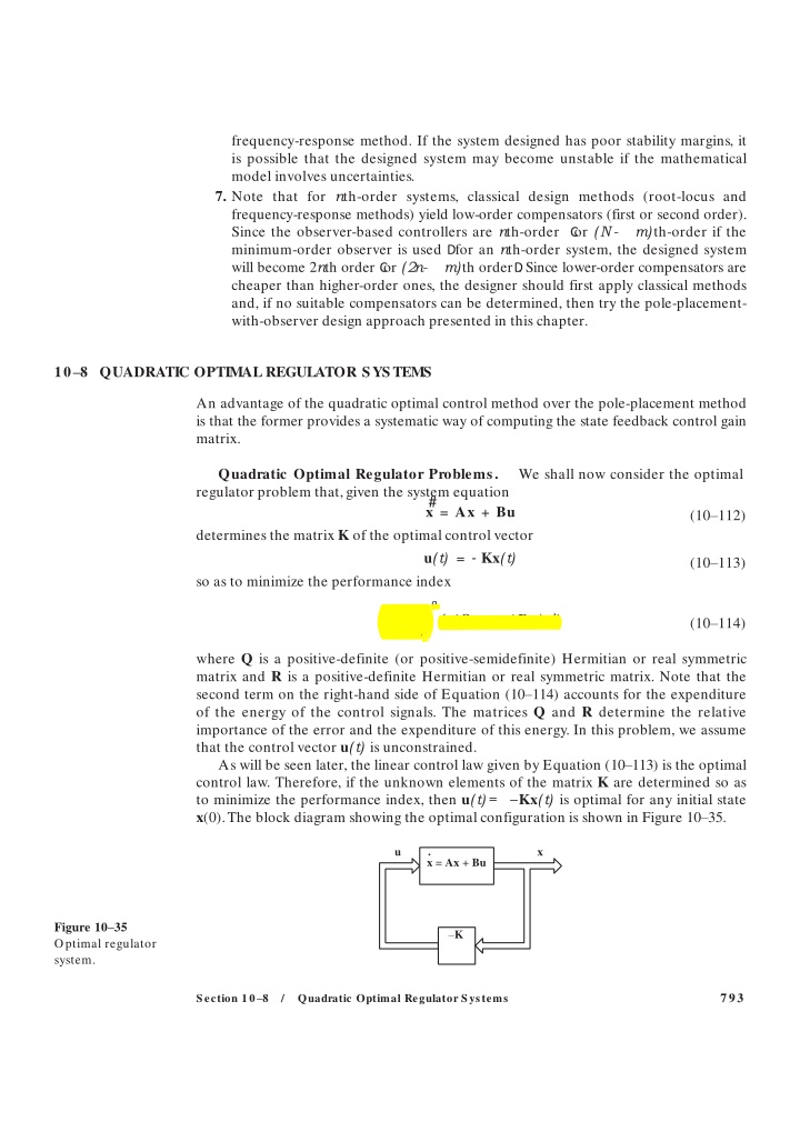
frequency-response method. If the system designed has poor stability margins, it is possible that the designed system may become unstable if the mathematical model involves uncertainties. 7. Note that for nth-order systems, classical design methods (root-locus and frequency-response methods) yield low-order compensators (first or second order). Since the observer-based controllers are nth-order C or (N- minimum-order observer is used Dfor an nth-order system, the designed system will become 2nth order C or (2n- m)th orderD . Since lower-order compensators are cheaper than higher-order ones, the designer should first apply classical methods and, if no suitable compensators can be determined, then try the pole-placement- with-observer design approach presented in this chapter. m)th-order if the 10 8 QUADRATIC OPTIMALREGULATOR SYSTEMS An advantage of the quadratic optimal control method over the pole-placement method is that the former provides a systematic way of computing the state feedback control gain matrix. Quadratic Optimal Regulator Problems. regulator problem that,given the system equation We shall now consider the optimal # x = Ax + Bu (10 112) determines the matrix K of the optimal control vector u(t) = - Kx(t) (10 113) so as to minimize the performance index q J = (x*Qx + u*Ru) dt (10 114) 30 where Q is a positive-definite (or positive-semidefinite) Hermitian or real symmetric matrix and R is a positive-definite Hermitian or real symmetric matrix. Note that the second term on the right-hand side of Equation (10 114) accounts for the expenditure of the energy of the control signals. The matrices Q and R determine the relative importance of the error and the expenditure of this energy. In this problem, we assume that the control vector u(t) is unconstrained. As will be seen later, the linear control law given by Equation (10 113) is the optimal control law. Therefore, if the unknown elements of the matrix K are determined so as to minimize the performance index, then u(t)= Kx(t) is optimal for any initial state x(0).The block diagram showing the optimal configuration is shown in Figure 10 35. . x = Ax + Bu u x Figure 10 35 Optimal regulator system. K 793 Section 10 8 / Quadratic Optimal Regulator Systems

Now let us solve the optimization problem. Substituting Equation (10113) into Equation (10 112),we obtain #x = Ax - BKx = (A - BK) x In the following derivations, we assume that the matrix A- eigenvalues of A- BK have negative real parts. SubstitutingEquation (10 113) into Equation (10 114) yields BK is stable, or that the q J = (x*Qx + x*K*RKx) dt 30 q = x*(Q + K*RK) xdt 30 Let us set d(x*Px) dt x*(Q + K*RK) x = - where P is a positive-definite Hermitian or real symmetric matrix.Then we obtain # x*(Q + K*RK) x = - x*Px - x*Px = - x*C (A - BK)*P + P(A - BK) D x # Comparingboth sidesof thislast equation and notingthat thisequation must hold true for any x,we require that (A - BK)*P + P(A - BK) = - (Q + K*RK) (10 115) It can be proved that if A- trix P that satisfies Equation (10 115).(See Problem A 10 15.) Hence our procedure is to determine the elements of P from Equation (10 115) and see if it is positive definite. (Note that more than one matrix P may satisfy this equation. If the system is stable, there always exists one positive-definite matrix P to satisfy this equation. This means that, if we solve this equation and find one positive-definite matrix P, the system is stable. Other P matrices that satisfy this equation are not positive definite and must be discarded.) The performance index J can be evaluated as BK is a stable matrix,there exists a positive-definite ma- q q x*(Q + K*RK)x dt = - x*Px2 J = = - x*( q ) Px( q ) + x*(0) Px(0) 30 0 Since all eigenvalues of A- x( q ) S 0.Therefore,we obtain BK are assumed to have negative real parts, we have J = x*(0) Px(0) (10 116) Thus, the performance index J can be obtained in terms of the initial condition x(0) and P. To obtain the solution to the quadratic optimal control problem, we proceed as follows: Since R has been assumed to be a positive-definite Hermitian or real symmetric matrix,we can write R = T*T 794 Chapter 10 / Control Systems Design in State Space

where T is a nonsingular matrix.Then Equation (10115) can be written as (A* - K*B*) P + P(A - BK) + Q + K*T*TK = 0 which can be rewritten as A*P + PA + C TK - (T*)- 1B*PD *C TK - (T*)- 1B*PD- PBR- 1B*P + Q = 0 The minimization of J with respect to K requires the minimization of x*C TK - (T*)- 1B*PD *C TK - (T*)- 1B*PD x with respect to K.(See Problem A 10 16.) Since thislast expression isnonnegative,the minimum occurs when it is zero,or when TK = (T*)- 1B*P Hence, K = T- 1(T*)- 1B*P = R- 1B*P (10 117) Equation (10 117) gives the optimal matrix K. Thus, the optimal control law to the quad- ratic optimal control problem when the performance index is given by Equation (10 114) is linear and is given by u(t) = - Kx(t) = - R- 1B*Px(t) The matrix P in Equation (10 117) must satisfy Equation (10 115) or the following reduced equation: A*P + PA - PBR- 1B*P + Q = 0 (10 118) Equation (10 118) is called the reduced-matrixRiccatiequation.The design steps may be stated as follows: 1. Solve Equation (10 118), the reduced-matrix Riccati equation, for the matrix P. [If a positive-definite matrix P exists (certain systems may not have a positive- definite matrix P),the system is stable,or matrix A- 2. Substitute this matrix P into Equation (10 117). The resulting matrix K is the optimal matrix. BK is stable.] A design example based on this approach is given in Example 10 9. Note that if the matrix A- BK is stable,the present method always gives the correct result. Finally, note that if the performance index is given in terms of the output vector rather than the state vector,that is, q J = (y*Qy + u*Ru) dt 30 then the index can be modified by using the output equation y = Cx to q J = (x*C*QCx + u*Ru) dt (10 119) 30 and the design steps presented in this section can be applied to obtain the optimal matrix K. 795 Section 10 8 / Quadratic Optimal Regulator Systems

EXAMPLE 109 Consider the system shown in Figure 10 36.Assuming the control signal to be u(t) = - Kx(t) determine the optimal feedback gain matrix K such that the following performance index is minimized: q A xTQx + u2Bdt J = 30 where Q = B1 0R 0) (m 0 m From Figure 10 36,we find that the state equation for the plant is # x = Ax + Bu where A = B0 1R , B = B0R 0 0 1 We shall demonstrate the use of the reduced-matrix Riccati equation in the design of the optimal control system. Let us solve Equation (10 118), rewritten as A*P + PA - PBR- 1B*P + Q = 0 Noting that matrix A is real and matrix Q is real symmetric, we see that matrix P is a real sym- metric matrix. Hence, this last equation can be written as 0 1 p11 p12 p p11 p 12 p12 p 0 0 R + B R B0 0R B1 0R Bp 22 12 22 R + B1 0R = B0 0R R B R[1][0 0 1]B p12 p11 p12 - p11 p12 B p22 p12 p22 1 0 m 0 0 This equation can be simplified to R + B1 R = B0 R + B0 p12p22 2 p11 p12R- p12 p12p22 0 0 0 0 m 0 Bp11 p12R 0 0 0 p222 B Plant u x2 x1 K Figure 10 36 Control system. 796 Chapter 10 / Control Systems Design in State Space

Plant u x2 x1 Figure 10 37 Optimal control of the plant shown in Figure 10 36. m + 2 ! from which we obtain the following three equations: 1 - p2= 0 12 p11- p12p22= 0 m + 2p - p = 0 2 12 22 Solving these three simultaneous equations for p11,p12,and p22,requiringP to be positive definite, we obtain P = Bp11 p12 p22 p12R = B 1 m + 2 1 R 1 m + 2 1 Referring to Equation (10 117),the optimal feedback gain matrix K is obtained as K = R- 1B*P 1]Bp11 p12R p22 = [1][0 p12 = C p12 p22D = C 1 1 m + 2D Thus, the optimal control signal is u = - Kx = - x1- 1 m + 2 x2 (10 120) Note that the control law given by Equation (10 120) yields an optimal result for any initial state under the given performance index. Figure 10 37 is the block diagram for this system. Since the characteristic equation is sI - A + BK = s2+ 1 m + 2 s + 1 = 0 if m= 1 , the two closed-loop poles are located at s = - 0.866 + j 0.5, s = - 0.866 - j 0.5 These correspond to the desired closed-loop poles when m= 1 . Solving Quadratic Optimal RegulatorProblems with MATLAB. the command In MATLAB, lqr(A,B,Q,R) 797 Section 10 8 / Quadratic Optimal Regulator Systems