Optimization of Media Criteria for Maximum Yield

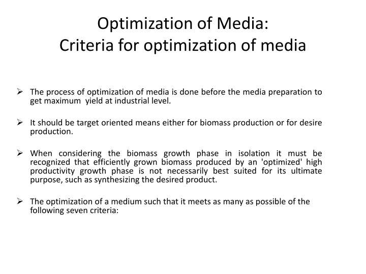
Optimization of Media: Criteria for optimization of media The process of optimization of media is done before the media preparation to get maximum yield at industrial level. It should be target oriented means either for biomass production or for desire production. When considering the biomass growth phase in isolation it must be recognized that efficiently grown biomass produced by an 'optimized' high productivity growth phase is not necessarily best suited for its ultimate purpose, such as synthesizing the desired product. The optimization of a medium such that it meets as many as possible of the following seven criteria:

1. 2. 3. 4. 5. 6. produce maximum yield of product or biomass per gram of substrate used. produce the maximum concentration of product or biomass. permit the maximum rate of product formation. give the minimum yield of undesired products. has consistent quality be readily available throughout the year. 7. It will cause minimal problems during -media making and -sterilization 8. It will cause minimal problems in other aspects of the production process particularly in -aeration and agitation, -extraction, -purification and -waste treatment.

Methods of optimization of media Classical Method The Plackett-Burman design

Classical Method Medium optimization by the classical method involve changing one independent variable (nutrient, antifoam, pH, temperature, etc.) while fixing all the others at certain level can be extremely time consuming expensive for a large number of variables.

Each possible combination of independent variable at appropriate levels could require a large number of experiments, xnwhere x is the number of levels and n is the number of variables.

This may be quite appropriate for three nutrients at two concentrations (2 3 trials) but not for six nutrients at three concentrations.In this instance 36(729) trials would be needed.

Industrially the aim is to perform the minimum number determine optimal alternative strategies considered which allow more than one variable to be changed at a time of experiments conditions. must therefore to Other be

The Plackett-Burman design When more than five independent variables are to be investigated, the Plackett-Burman design may be used to find the most important variables in a system, which are then optimized in further studies.

This technique allows for the evaluation of X-I variables by X experiments. X must be a multiple of 4, e.g. 8, 12, 16, 20, 24, etc.

Normally one determines how many experimental variables need to be included in an investigation and then selects the Plackett-Burman design which meets that requirement most closely in multiples of 4. Any factors not assigned to a variable can be designated as a dummy variable. And factors known to not have any effect may be included and designated as dummy variables

Table 4.16 shows a Plackett-Burman design for seven variables (A -G) at high and low levels in which two factors, E and G, are designated as 'dummy' variables. From Principles of Fermentation Technology,- Peter F. Stanbury, Allen Whitaker, Stephen J. Hall, Second Edition,

Each horizontal row represents a trial and each vertical column represents the H (high) and L (low) values of one variable in all the trials. The effects of the dummy variables are calculated in the same way as the effects of the experimental variables. If there are no interactions and no errors in measuring the response, the effect shown by a dummy variable should be O. If the effect is not equal to 0, it is assumed to be a measure of the lack of experimental precision plus any analytical error in measuring the Response.

From Principles of Fermentation Technology,- Peter F. Stanbury, Allen Whitaker, Stephen J. Hall, Second Edition,

The stages in analysing the data (Tables 4.16 and 4.17) using Nelson's (1982) example are as follows: 1. Determine the difference between the average of the H (high) and L (low) responses for each independent and dummy variable. Therefore the difference = LA (H) - LA (L).

The effect of an independent variable on the response is the difference between the average response for the four experiments at the high level and the average value for four experiments at the low level. Thus the effect of This value would be near zero for the dummy variables

2. Estimate the mean square of each variable (the variance of effect). For A the mean square will be = 3. The experimental error can be calculated by averaging the mean squares of the dummy effects of E and G. Thus, the mean square for error = This experimental error is not significant.

4. The final stage is to identify the factors which are showing large effects. In the example this was done using an F-test for Factor mean square. error mean square. When Probability Tables are examined it is found that Factors A, Band F show large effects which are very significant, whereas C shows a very low effect which is not significant and D shows no effect. A, B and F have been identified as the most important factors.