Optimizing Asynchronous Transfer Line for Circuit Board Assembly
Explore the design process of a new 4-workstation assembly line for circuit board assembly, focusing on selecting technology options and minimizing deployment costs while meeting production requirements. Various scenarios, including baseline designs, reducing cycle time, and adding capacity to stations, are analyzed for efficiency and cost-effectiveness.

Download Presentation

Please find below an Image/Link to download the presentation.
The content on the website is provided AS IS for your information and personal use only. It may not be sold, licensed, or shared on other websites without obtaining consent from the author. If you encounter any issues during the download, it is possible that the publisher has removed the file from their server.
You are allowed to download the files provided on this website for personal or commercial use, subject to the condition that they are used lawfully. All files are the property of their respective owners.
The content on the website is provided AS IS for your information and personal use only. It may not be sold, licensed, or shared on other websites without obtaining consent from the author.
E N D
Presentation Transcript
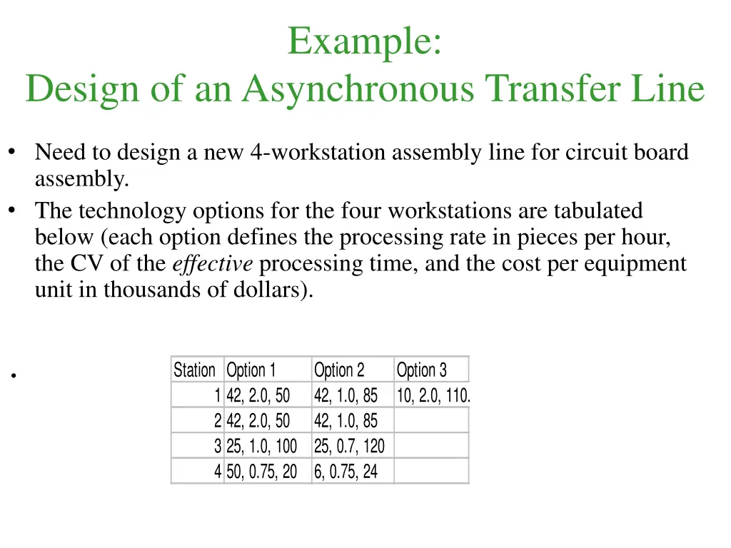
Example: Design of an Asynchronous Transfer Line Need to design a new 4-workstation assembly line for circuit board assembly. The technology options for the four workstations are tabulated below (each option defines the processing rate in pieces per hour, the CV of the effective processing time, and the cost per equipment unit in thousands of dollars). Station Option 1 1 42, 2.0, 50 2 42, 2.0, 50 3 25, 1.0, 100 4 50, 0.75, 20 Option 2 42, 1.0, 85 42, 1.0, 85 25, 0.7, 120 6, 0.75, 24 Option 3 10, 2.0, 110.5
Example: ATL Design (cont.) Each workstation can employ only one technology option. The maximum production rate to be supported by the line is 1000 panels / day. The desired average cycle time through the line is one day. One day is equivalent to an 8-hour shift. Workpieces will go through the line in totes of 50 panels each, which will be released into the line at a constant rate determined by the target production rate. We want to select the technology options for the line workstations and the number of units from the corresponding technologies in order to minimize the deployment cost of the line.
A baseline design:Meeting the desired prod. rate with a low cost 1000 42,2.0,50 42,1.0,85 8 10,2.0,110.5 42,2.0,50 42,1.0,85 25,1.0,100 25, 0.7,120 50,0.75,20 6,0.75,24 50 (1000 / 50) / 8 2.5 Station 1 Station 2 Station 3 Station 4 1/te Ce P m 42 2 50 3 42 2 50 3 25 1 50 0.75 20 100 6 3 te 0.0238 1.1905 0.08 0.9921 0.0238 1.1905 0.08 0.9921 0.04 0.02 tb=B*te Cb^2=Ce^2/B u=TH*tb/m 2 1 0.02 0.0113 0.8333 0.8333 Ca^2 0 0.4615 0.4687 0.4687 0.5598 0.5598 0.4691 Cd^2 = 1+(1-u^2)(Ca^2-1)+(u^2/sqrt(m))*(Cb^2-1) 0.4615 CT = [(Ca^2+Cb^2)/2]*[u^(sqrt(2*(m+1))-1)/(m*(1-u))]*tb+tb CT1+CT2+CT3+CT4 WIPq 3.17 14.6 2.3 1.41 21.48 4.9 33.5 0.8 1 m*P 150 150 600 60 960
Reducing the line cycle time by adding capacity to Station 2 1000 42,2.0,50 42,1.0,85 8 10,2.0,110.5 42,2.0,50 42,1.0,85 25,1.0,100 25, 0.7,120 50,0.75,20 6,0.75,24 50 (1000 / 50) / 8 2.5 Station 1 Station 2 Station 3 Station 4 1/te Ce P m 42 2 50 3 42 2 50 4 25 1 50 0.75 20 100 6 3 te 0.0238 1.1905 0.08 0.9921 0.0238 1.1905 0.08 0.7441 0.04 0.02 tb=B*te Cb^2=Ce^2/B u=TH*tb/m 2 1 0.02 0.0113 0.8333 0.8333 Ca^2 0 0.4615 0.505 0.505 0.5709 0.5709 0.4725 Cd^2 = 1+(1-u^2)(Ca^2-1)+(u^2/sqrt(m))*(Cb^2-1) 0.4615 CT = [(Ca^2+Cb^2)/2]*[u^(sqrt(2*(m+1))-1)/(m*(1-u))]*tb+tb CT1+CT2+CT3+CT4 WIPq 3.17 1.36 2.32 1.42 8.27 1.1 4.9 0.4 0.8 m*P 150 200 600 60 1010
Adding capacity at Station 1, the new bottleneck 1000 42,2.0,50 42,1.0,85 8 10,2.0,110.5 42,2.0,50 42,1.0,85 25,1.0,100 25, 0.7,120 50,0.75,20 6,0.75,24 50 (1000 / 50) / 8 2.5 Station 1 Station 2 Station 3 Station 4 1/te Ce P m 42 2 50 4 42 2 50 4 25 1 50 0.75 20 100 6 3 te 0.0238 1.1905 0.08 0.7441 0.0238 1.1905 0.08 0.7441 0.04 0.02 tb=B*te Cb^2=Ce^2/B u=TH*tb/m 2 1 0.02 0.0113 0.8333 0.8333 Ca^2 0 0.299 0.4324 0.4324 0.5487 0.5487 0.4657 Cd^2 = 1+(1-u^2)(Ca^2-1)+(u^2/sqrt(m))*(Cb^2-1) 0.299 CT = [(Ca^2+Cb^2)/2]*[u^(sqrt(2*(m+1))-1)/(m*(1-u))]*tb+tb CT1+CT2+CT3+CT4 WIPq 1.22 1.31 2.27 1.4 6.2 0.1 0.3 0.7 1 m*P 200 200 600 60 1060
An alternative option:Employ less variable machines at Station 1 1000 42,2.0,50 42,1.0,85 8 10,2.0,110.5 42,2.0,50 42,1.0,85 25,1.0,100 25, 0.7,120 50,0.75,20 6,0.75,24 50 (1000 / 50) / 8 2.5 Station 1 Station 2 Station 3 Station 4 1/te Ce P m 42 1 85 3 42 2 50 4 25 1 50 0.75 20 100 6 3 te 0.0238 1.1905 0.02 0.9921 0.0238 1.1905 0.08 0.7441 0.04 0.02 tb=B*te Cb^2=Ce^2/B u=TH*tb/m 2 1 0.02 0.0113 0.8333 0.8333 Ca^2 0 0.4274 0.4897 0.4897 0.5662 0.5662 0.4711 Cd^2 = 1+(1-u^2)(Ca^2-1)+(u^2/sqrt(m))*(Cb^2-1) 0.4274 CT = [(Ca^2+Cb^2)/2]*[u^(sqrt(2*(m+1))-1)/(m*(1-u))]*tb+tb CT1+CT2+CT3+CT4 WIPq 1.69 1.35 2.31 1.41 6.76 1.2 0.4 0.8 1 m*P 255 200 600 60 1115 This option is dominated by the previous one since it presents a higher CT and also a higher deployment cost. However, final selection(s) must be assessed and validated through simulation.

")