Optimizing Gravity-Sustained Water Distribution Systems

Slide Note

Creating an efficient water distribution system involves optimizing pipe diameters, considering energy loss, pressure constraints, and velocity limits. This process requires iterative calculations to find the best solution and ensure reliable water supply to all points. Learn more about the design and optimization of gravity-sustained distribution mains.

bay_bur Follow

Uploaded on Feb 22, 2025 | 0 Views

Download Presentation

Please find below an Image/Link to download the presentation.

The content on the website is provided AS IS for your information and personal use only. It may not be sold, licensed, or shared on other websites without obtaining consent from the author.If you encounter any issues during the download, it is possible that the publisher has removed the file from their server.

You are allowed to download the files provided on this website for personal or commercial use, subject to the condition that they are used lawfully. All files are the property of their respective owners.

Download Presentation

The content on the website is provided AS IS for your information and personal use only. It may not be sold, licensed, or shared on other websites without obtaining consent from the author.

E N D

Presentation Transcript

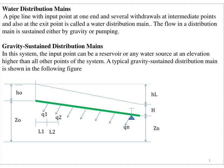
Water Distribution Mains A pipe line with input point at one end and several withdrawals at intermediate points and also at the exit point is called a water distribution main.. The flow in a distribution main is sustained either by gravity or pumping. Gravity-Sustained Distribution Mains In this system, the input point can be a reservoir or any water source at an elevation higher than all other points of the system. A typical gravity-sustained distribution main is shown in the following figure ho hL H q1 q2 Zo qn Zn L1 L2 1

The total energy loss is equal to the available potential head ? 8??????2 ?2???5 ??+ ??+ ? = 0 ?=1 2 0.9 ? ?? ?? ? = 1.325 ?? + 4.618 3.7 ?? The optimal diameter for every reach is 0.2 ? ? 8 1 ??????2 ?? = (????2) ?+5 ?2?(?? ?? ?) ?+5 ?=1 The above equation calculates optimal pipe diameters assuming constant friction factor. Thus the diameters obtained using arbitrary values of f are approximate. These diameters can be improved by evaluating f using the equation of friction factor and estimating a new set of diameters by the above equations. The procedure can be repeated until the two successive solutions are close. The design should be checked against the minimum and maximum pressure constraints at all nodal points. The design should also be checked against the maximum velocity constraint. 2

Example : Design a gravity-sustained distribution main with the following data, m = 0.935 , = ?.?? ?? , H= 5 m Demand discharge, qi, ?3/? Pipe Pipe Zi L, m Discharge , Qi, ?3/s 0 1 2 3 4 5 100 94 92 89 88 87 1500 200 1000 1500 500 0.01 0.015 0.02 0.01 0.01 0.065 0.055 0.04 0.02 0.01 Solution: Assume f1=f2=f3=f4=f5=0.01 3

First Iteration ??????20.1575 307.015 38.837 175.65 211.795 56.751 790.048 Pipe No. ?? ?? ?? 1 2 3 4 5 1500 200 1000 1500 500 0.01 0.01 0.01 0.01 0.01 0.065 0.055 0.04 0.02 0.01 Sum ??= ????20.1685 1.5217 ????20.1685 Pipe No. ?? 1 2 3 4 5 0.183 0.173 0.156 0.123 0.0975 0.279 0.264 0.237 0.187 0.148 0.02031 0.02065 0.02131 0.02291 0.02474 4

Second Iteration ??????20.1575 343.26 43.536 197.879 241.335 65.453 891.463 Pipe No. ?? ?? ?? 1 2 3 4 5 1500 200 1000 1500 500 0.02031 0.02065 0.02131 0.02291 0.02474 Sum 0.065 0.055 0.04 0.02 0.01 ??= ????20.1685 1.5217 ????20.1685 Pipe No. ?? 1 2 3 4 5 0.2064 0.1957 0.1767 0.1416 0.1136 0.322 0.305 0.275 0.221 0.177 0.0199 0.02026 0.02092 0.02251 0.02435 5

Third Iteration ??????20.1575 342.159 43.516 197.305 240.666 65.2895 888.936 Pipe No. ?? ?? ?? 1 2 3 4 5 1500 200 1000 1500 500 0.0199 0.02026 0.02092 0.02251 0.02435 Sum 0.065 0.055 0.04 0.02 0.01 ??= ????20.1685 1.5217 ????20.1685 Pipe No. ?? 1 2 3 4 5 0.2057 0.1956 0.1762 0.1412 0.1133 0.321 0.305 0.274 0.220 0.177 0.0199 0.02026 0.02093 0.02252 0.02435 The difference between the successive values of diameters within the tolerance of limits. 6

Pumped Distribution Pumping distribution mains are provided for sustaining the flow if the elevation difference between the entry and exit points is very small, also if the exit point level or an intermediate withdrawal point level is higher than the entry point level, as shown in Fig. hf H ho q6 q5 Pump q4 q3 q2 Zn q1 Reservoir Zo L2 L1 The head loss constraint of the system is given by ? 8??????2 ?2???5 ?? ?+ ??+ ? = 0 7 ?=1

The optimal diameter is 1 40 ??????1??2 ?2??? ?+5 ?? = 5 ? ?2??? 40????1 ? ?+5 8 = ??+ ? ??+ ??????2 ?+5 ? ?2? ?=1 Example : Design a pump distribution main using the following data, the terminal pressure head is 5 m. Adopt cast iron pipe for the design , m= 0.935, ?? ??= 0.02, = 0.25 ??. Demand Discharge, ?3/? Pipe Discharge, ?3/? Pipe Zi L, m 0 1 2 3 4 5 100 102 103 105 106 109 1200 500 1000 1500 700 0.012 0.015 0.015 0.02 0.014 0.076 0.064 0.049 0.034 0.014 8

First Iteration Assume f= 0.01 for all reaches ??= 6.58859 ????20.16849 0.265 0.25 0.229 0.202 0.15 Pipe fi Qi fi 1 2 3 4 5 0.01 0.01 0.01 0.01 0.01 0.076 0.064 0.049 0.034 0.014 0.0203 0.0207 0.0212 0.022 0.0241 Second Iteration ??= 6.58859 ????20.16849 0.299 0.283 0.26 0.231 0.174 Pipe fi Qi fi 1 2 3 4 5 0.0203 0.0207 0.0212 0.022 0.0241 0.076 0.064 0.049 0.034 0.014 0.020 0.0203 0.0208 0.0216 0.0237 9

Third Iteration ??= 6.58859 ????20.16849 0.298 0.282 0.259 0.23 0.174 Pipe fi Qi fi 1 2 3 4 5 0.020 0.0203 0.0208 0.0216 0.0237 0.076 0.064 0.049 0.034 0.014 0.02 0.0203 0.0208 0.0216 0.0237 Calculate ? ??????20.1575 287.773 113.854 210.139 282.607 101.193 995.566 Pipe fi Qi Li 1 2 3 4 5 0.020 0.0203 0.0208 0.0216 0.0237 0.076 0.064 0.049 0.034 0.014 Sum 1200 500 1000 1500 700 10