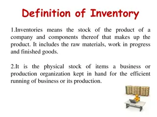
Explore the advantages of periodic review inventory control policies, including order-up-to and (s, S) policies. Understand key concepts such as safety stocks, service levels, and average inventory levels for efficient inventory management. Discover examples and calculations to help you implement the right strategy for your business needs.
Please find below an Image/Link to download the presentation.
The content on the website is provided AS IS for your information and personal use only. It may not be sold, licensed, or shared on other websites without obtaining consent from the author. If you encounter any issues during the download, it is possible that the publisher has removed the file from their server.
You are allowed to download the files provided on this website for personal or commercial use, subject to the condition that they are used lawfully. All files are the property of their respective owners.
The content on the website is provided AS IS for your information and personal use only. It may not be sold, licensed, or shared on other websites without obtaining consent from the author.
E N D
Presentation Transcript
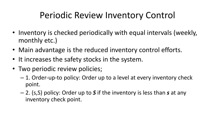
Periodic Review Inventory Control Inventory is checked periodically with equal intervals (weekly, monthly etc.) Main advantage is the reduced inventory control efforts. It increases the safety stocks in the system. Two periodic review policies; 1. Order-up-to policy: Order up to a level at every inventory check point. 2. (s,S) policy: Order up to S if the inventory is less than s at any inventory check point.
Periodic review; order-up-to policy OUL Q1 Q3 Q2 Covered time span by OUL = T + T T What is the right value for OUL ? OUL covers the demand from A to D or from C to F.
Periodic review; order-up-to policy OUL should protect the system against running out of inventory during T + periods. Random = + OUL + periods level) demand ) = during service (cycle T D Pr + D T ( T If the demand during T + follows a normal distribution std. deviation of demand during T + = ++ z OUL + T T safety stock mean demand during T +
Periodic review; order-up-to policy std. deviation of demand during T + = ++ z OUL + T T safety stock mean demand during T + = + = + ( T ) T , + T p + T std. deviation of demand in a period exp. demand in a period Q =2 + inventory . Av s T = Q p
Periodic review; order-up-to policy Example: Wallmart ordering Rego Weekly demand ~N Lead time = 2 weeks Wallmart applies a monthly periodic MU-control policy (T = 4 weeks) Wallmart determindes that cycle service level to be equal to = 0.9 OUL=? Safety stock? Average inventory? = = ( 2500 , 500 ) H H
Periodic review; order-up-to policy weeks 6 2 4 T = + = + + = + T = = T H 6 2500 15000 units 6 = + T + T = = 6 500 1225 unit 6 = + = 1225 ) 28 . 1 ( + = 15000 16568 OUL z 6 0.9 6 Average inventory level = ? ?+ ? Q = 4 2500 = 10000 Average inventory = ????? + 1568 = 6568 ?
Periodic review; order-up-to policy What if Wallmart used a continuous review policy? Safety stock? = + . 1 = 28 2 500 905 units s z (665 less safety stock compared to the periodic review policy) There are some other periodic review policy. For example (s, S) policy = + s = R S R Q
Alternative Periodic Review Policy: (s, S) Policy Define two levels, s < S, and let u be the starting inventory at the beginning of a period. Then, if u is less or equal to s, order (S u), if u is more than s, do not place an order. In general, computing the optimal values of s and S is difficult. Approximation: Compute optimal values for (Q,R) model and then set; s = R , S = R + Q , T=Q/
Periodic review v.s. Continuous review model Periodic Continuous Fixed ordering times, random order quantity Long protection periods against uncertainty Larger safety stock for the same cycle service level Less effort for control Particularly suited for consolidating different items ordered from the same supplier Fixed order sizes, random times between orders Short protection period against uncertainty Less safety stock More effort for controlling inventory Difficult to consolidate the orders
Single period stochastic inventory problem The problem is called newsboy problem; A newsboy must decide the number of newspapers to buy at the beginning of the day Observes the demand during day At the end of the day newsboy either Runs out of newspapers and loses some sales or Ends up with some unsold newspapers and gets rid of them, therefore, looses some money Decision; How many newspapers to order?
Single period stochastic inventory problem Almost all retailers faces this problem every season (summer, winter) Many products have a model for summer or winter season (typical examples are fashion products.) A similar problem has to be solved for some service industries; How many seats in a flight should be allocated to discounted tickets that will be purchased in advance? How many rooms in a hotel to be reserved for early reservation versus walk-ins? How many mid-size cars to have for a rental company in the summer season?
Newsboy problem - Example A newsboy is selling the weekly magazine, The computer journal Observed demand in the past 52 weeks 15 19 14 11 8 6 8 11 11 18 15 17 19 14 14 17 13 12 9 12 6 11 5 9 22 9 18 10 4 17 18 14 15 9 10 4 7 1 14 12 8 11 9 7 12 15 15 19 4 8 9 16 Avr = 11.7 std=4.74 The newsboy buys each copy for $0.25 and sells it for $0.75 At end of the week he can return each unsold copy for $0.10 Question: How many copies to buy at the beginning of the week? Average? More than the average?
Newsboy problem - Example The cost of each issue unsold? Called cost of overage Purchase price (c) salvage value (s) ; c s = 0,25 - 0,1 = 0.15 $ The lost profit due to lost customer? Called cost of underage Selling price (p) purchase price (c) ; p c = 0,75 - 0,25 = 0,5 $ Intuition tells us to order more than the average. But how much more?
Newsboy problem modeling environment Relatively short selling season (weeks, 4 months etc.) with a well-defined beginning and end At the beginning of the period, a decision is made on how much to order or produce (Q) The demand (D) is uncertain, we have a forecast on its distribution (empirical or theoretical) F(X)= P(D<=X); the cumulative distribution function (cdf) of D f(x); Probability density function (pdf) of D
Newsboy problem modeling environment When the total demand in the period exceeds the stock available, there is an associated underage cost, cu cost per unit of unsatisfied demand When the total demand is less than the stock available, overage cost is incurred, co cost per unit of positive inventory at the end of the period Objective: Minimize the total underage and overage cost in a season = Maximizing the expected profit in a season
Development of the cost function Define G(Q,D) as the total overage and underage cost incurred at the end of the season when Q units are ordered and the realized demand is D = + G ( Q , D = ) c max{ , 0 Q Expected cost of ordering Q D } c max{ , 0 D Q } o u G ( Q ) E [ G ( Q , D )] = + c max{ , 0 Q x } f ( x ) dx c max{ , 0 x Q } f ( x ) dx o u 0 0 Q = + c ( Q x ) f ( x ) dx c ( x Q ) f ( x ) dx o u 0 Q
Finding the optimal order size Necessary condition for the optimal order size; Q = ( ) 0 G Derivative of the integral using Leibniz s Rule; ( ) b Q ( d = Q ( , ) g x dx dQ ) a Q ( ) b Q ( ( , ) d d dg x Q + Q ( ) Q ( , Q ( )) Q ( ) Q ( , Q ( )) b g b a g a dx dQ dQ dQ ) a Q
Finding the optimal order size Q ( ) dG Q = + ) 1 1 ( ) ( ( ) c f x dx c f x dx o u dQ 0 Q = ( ) 1 ( u ( )) c F Q c F Q o The function is convex (the second order condition is satisfied) 2 ( ) d G Q = + ( ) ( ) 0 c c f Q o u X 2 dQ = + = ' * * ( ) ( ) ( ) 0 G Q c c F Q c o u u c = The = * ( ) critical ratio (cr) u F Q + c c o u
Understanding the critical ratio The critical ratio (CR) is targeted optimal probability of not having any lost sale = Optimal customer service level c + u CR= Area = c c u o Qcr
Understanding the critical ratio When; Cu =Co and the demand distribution is symmetric Order the average demand A nitch market, fashion product with high profit margin => Cu is very large High customer service level is targeted Very much of a commodity product with low profit margin => Cu is low Lower customer service level is targeted Targeted optimal service level depends on the product type
Normally Distributed Demand Demand s normal distribution Standard normal distribution c + u Area = (z ) c c u o z D D 0 Qcr Zcr = = 0 1 Q = . . c r D Z cr D = + . Q Z . cr D c r D 21
Back to the Newsboy Example 5 , 0 + c + = = = 0 77 . u F(Q*) 5 , 0 0 15 . c c u o Z0,77= NORMSINV(0.77) = 0.74 (Excel function) 0.09 = + Q* z 0.08 0.07 0.06 Probability 0.05 =11.73+ (0.74*4.74) =15,24 ~ order 15 magazines 0.04 0.03 0.02 0.01 0 1 2 3 4 5 6 7 8 9 10 11 12 13 14 15 16 17 18 19 20 21 22 Sales Area=0.77
Extention of the example: zero value for an unsold item Assume now that the newsboy cannot return the unsold copies to the publisher. In this case, Co = 0,25-0 = 0,25 CR = 0,5/(0,5+0,25) = 0.667 0.09 0.08 Z0,667=0,431 0.07 0.06 Probability 0.05 0.04 We will order less since it is now more costly to have excess inventory 0.03 0.02 0.01 0 1 2 3 4 5 6 7 8 9 10 11 12 13 14 15 16 17 18 19 20 21 22 Sales Q=11.73+ (0.431*4.74) =13,77 ~ order 14 magazines Area= 0.667
Extention of the example: Uniform demand distribution What if the demand distribution is uniform between 8 and 20. 1 8 20 if x = OW ( ) f x 20 8 F(X) 0 f(x) 0 8 if x 8 x = X 8 20 ( ) 8 20 F x if x if 20 8 1 20 x * 8 Q = = = * ( ) , 0 77 F Q CR 20 8 + = = * , 0 77 12 ( ) 8 17 , 24 17 magazines Q
Emprical (discrete) distribution case Demand data for the last 52 weeks 15 19 14 11 8 6 8 11 11 18 15 17 19 14 14 17 13 12 - In the previous analysis we have assumed that the demand follows a normal distribution and we estimated the mean and standard deviation of the distribution -1 How accurately the normal distribution represent the data ? (Histogram, Normality plot, Chi-square test) - 2 How accurate are our estimations of the mean and standard deviations? 9 12 6 11 5 9 22 9 18 10 4 17 18 14 15 9 10 4 7 0 14 12 8 11 9 7 12 15 15 19 4 8 9 16 - Alternative to normal distribution assumption: Use emprical distribution
Emprical (discrete) distribution case Demand Frequency Cumulative. Freq. Cumulative frequency column is the emprical distribution Example: F(3)=4/52 We need F(Q*)=CR=0,77. What Q* gives us 0,77 Cumulative Freq.? CR=0,77 is between; F(14)=0,69, F(15)=0,79 Set Q* to the upper value of the range always Q*= 15 is the solution here. 0 1 2 3 . . 14 15 . . 22 1/52 0 0 3/52 . . 6/52 5/52 . . 1/52 1/52 1/52 1/52 4/52 . . 36/52=0,69 41/59=0,79 . . 52/52
Pros and Cons of using Emprical distributions Pros Very easy to construct Can be used with any data where none of the theoretical distribution fits the data No error due to estimating the distribution and its parameters Cons It will have irregularities which may not be representing the data It is based on the limited amount of data. With each additional data, we will have somewhat different distribution.
Extention to regular newsboy model: A more complicated cost case Example: We buy and sell winter coats Purcase price c=35 TL Selling price P=65 TL All the leftover inventory at the end of the season are sold at the outlet with 55% discount Inventory holding cost per season 5% Transportation cost to the outlet is 1$/coat What are Co and Cu ?
Extention to regular newsboy model: A more complicated cost case Salvage value (s) s = selling price of the left over transportation cost inventory holding cost s = 65 (1-0,55) 1 35(0,05) = 26,5TL/coat Co=c-s = 35 26,5 = 8,5 TL Cu= p-s = 65 35 = 30 TL We calculate CR and obtain Q* in the same way as before.
Extention to regular newsboy model: A more complicated cost case What if we have an emergency supply option from a local, fast supplier, in case there is a any shortage with a price of 50 TL/coat? Co, Cu? Co is the same as before. Cu = Emergency purchase price Normal purchase price = 50 35 = 15 TL
Histogram in Excel Constructing Histogram in excel Veri > Veri z mleme > histogram Indicate the data range Indicate the bin range for grouping data (optional, if not provided, excel will decide the grouping). Suggested number of bins = Number of data points Bin size = (maximum-minimum)/No. Bins Bin ranges: First bin = minimum + Bin size Increment each bin by bin size Enter a workbook name for output Click on the k m latif y zde and grafik kt s
Histogram in Excel; Obtaining Empirical distribution Constructing Histogram in excel for emprical distribution; Veri > Veri z mleme > histogram Indicate the data range Indicate the bin range for grouping data. Bins; From the minimum data till the maximum data, incremented by one (one bin for each value in the data). Enter a workbook name for output Click on the k m latif y zde and grafik kt s
Normal distribution Histogram 25 120.00% 100.00% 20 80.00% 15 Frekans 60.00% 10 Frekans 40.00% K m latif % 5 20.00% 0 0.00% Bin If the data is normally distributed; - Bell shaped higtogram - S shaped cumulative distribution
Inventory-related metrics Inventory turns a year = Total annual sales (or use)/average inv. Number of orders per unit time (e.g. Per year or month). Fill rate: fraction of demand/orders satisfied from inventory Cycle service level: Fraction of cycles we are not out of stock. Safety inventory: average inventory when the replenishment order arrives. Average inventory; measured in units, financial value, or days of demand. Average replenishment batch size; measured by SKU (stock keeping unit) in terms of both units and days of demand.
How to reduce inventories? Reduce fixed costs of ordering/set up IT technologies (RFID, El. Data Interchange), automated ordering systems, high tech storage systems, single minute exchange of dies (SMED) Reduce the safety stock Reduce the expected value of lead time Reduce the variability of lead time Apply continuous monitoring rahter than periodic review as much as possible
ABC classification in multi item inventory control Classifying the inventoried items based on their importance and allocating the control effort based on this importance classification Importance: Annual dollar volume of items sold/used Note: Importance could be defined in different ways A spare part for a machine which is a bottleneck in the manufacturing process A cheap component but if we run out of stock in this component we must stop the entire assembly line
ABC classification in multi item inventory control In the classification pareto rule usually applies and we find a plot similar to the one below Annual sale/usage ($) A 60%- 80% B 15%- 30% C 5-10% 50% 15% 35% Item types (%)
ABC classification 14 chemical products in the inventory of a retail store Item Type % (Rank/14) Total Sale % 36.2% 60.7 Sale volume rank ABC Annual Sale $5,056 3,424 - ID D-204 D-212 classification 1 2 7.1% 14.3 A (14.3%) D-1850 D-191 D-192 D-193 D-179 -0 3 4 5 6 7 1,052 893 843 727 451 68.3 74.6 80.7 85.7 89.1 21.4 28.6 35.7 42.9 50.0 B (35.7%) D-195 D-196 D-186 -0 D-198 - D-199 D-200 D-205 8 9 412 214 205 188 172 170 159 91.9 93.6 95.1 96.4 97.6 98.7 100.0 57.1 64.3 71.4 78.6 85. 7 92.9 100.0 10 11 12 13 14 C (50%) $13,966 CR (2004) Prentice Hall, Inc. 3-5
80-20 plot 100 90 Toplam sat (%) 80 70 60 50 40 30 A r nleri B r nleri C r nleri 20 10 0 0 20 40 60 80 100 Toplam r n (%) CR (2004) Prentice Hall, Inc. 3-6
ABC classification in multi item inventory control Continuous reviewing for the stock levels More sophisticated forecasting procedures should be used Cost parameters should be carefully estimated (to determine the best ordering policy) For type A items The inventories can be reviewed periodically Items can be ordered in groups rather than individually Less sophisticated forecasting methods can be used For B type items Minimum degree of control ! For very inexpensive items, order large lot sizes For expensive C items with low demand, do not hold any inventory For type C items


")


 distribution case")
 distribution case")