Explore the Controller Area Network (CAN) history, protocol details, error detection mechanisms, and scheduling model. Understand how CAN revolutionized automotive communication systems with its efficient data transfer methods and real-time message handling. Dive into the development timeline and significance of CAN in modern vehicles.
Please find below an Image/Link to download the presentation.
The content on the website is provided AS IS for your information and personal use only. It may not be sold, licensed, or shared on other websites without obtaining consent from the author. If you encounter any issues during the download, it is possible that the publisher has removed the file from their server.
You are allowed to download the files provided on this website for personal or commercial use, subject to the condition that they are used lawfully. All files are the property of their respective owners.
The content on the website is provided AS IS for your information and personal use only. It may not be sold, licensed, or shared on other websites without obtaining consent from the author.
Outline Recap on CAN Scheduling Model Schedulability Results
Recap on CAN Controller Area Network A multi-master serial data bus which uses Carrier Sense Multiple Access/Collision Resolution to determine access.
History of CAN on automotive Developed in 1983; first controller chip by Intel and Philips in 1987; ISO standard in 1993. Mercedes was the first to deploy CAN in a production car (1993). In mid 1990s, number of ECUs grew rapidly. As a result, point-to-point wiring became impractical (lots of copper wire). CAN started to be adopted as the solution to increase electronics content. By 2004, over 50 different microprocessor families with on-chip CAN capability. The Environmental Protection Agency mandated the use of CAN in all cars from model year 2008 onwards.
A brief look at CAN protocal Message transfer over CAN is controlled by 4 types of frame: data frames remote transmit request frames overload frames error frames Normally, CAN nodes (ECUs) are only allowed to start transmitting when the bus is idle. Different CAN nodes may not have synchronized clocks. So nodes will re-synchronize through the start of frame bit on each message transmission.
Error Detection 15-bit Cyclic Redundancy Check is used to check errors in the transmitted messages. When error detected, the node sends error flag 000000 or 111111 . The transmission of an error flag usual causes other nodes to also detect the error. Since bit patterns 000000 and 111111 have special meanings, we need to avoid them in the variable part of the transmitted messages.
Bit Stuffing Bit-stuffing: A bit of the opposite polarity is inserted by the transmitter whenever 5 bits of the same polarity are transmitted. This process is reversed by the receiver. Example:
Scheduling Model The system is comprised of a number of nodes (microprocessors) connected via CAN. The system is assumed to contain a static set of hard real-time messages. Each message m is statically assigned to a node. Each message m has a fixed identifier (thus a unique priority), and each node attempts to transmit the highest priority message queued at that node.
Scheduling Model (cont.) Each message has a max number of data bytes sm and max transmission time Cm. Each message is assumed to be queued by a software task (triggered by events). To account for the clock drift due to the lack of synchronized clock, this task needs a bounded amount of time between 0 and Jmto queue a message ready for transmission. Jmis referred as queuing jitter. The event that triggers the queuing of message m is assumed to occur with a min inter-arrival time of Tm, referred as period.
Scheduling Model (cont.) Each message m has a hard deadline Dm, corresponding to the max permitted time from the occurrence of the triggering event to the end of successful transmission of the message, i.e. all nodes require m have received it. Receiving nodes may have different timing requirements, and we assume Dmto be the tightest. The worst-case response time Rm. Message m is scheduable iff Rm Dm.
Summary of Scheduling Model Messages are sent as if all the nodes on the network shared a single global priority-based queue. Messages are sent on the bus according to a fixed priority non-preemptive schedule. However, the real timing behavior of CAN in an actual system can be much more complicated.
Survey of Related Scheduling Result Before Tindell et al. (1994), there is a misconception about CAN that Transmitting highest priority message with low latency Not possible to guarantee less urgent signals -> low priority messages would miss their deadlines. Tindell s paper provides a Worst-Case Response Time bound based on uniprocessor fixed-priority preemptive scheduling. Prior to Tindell s work, bus utilization was in 30% - 40%. After, bus utilization raised to 80%.
Survey of Related Scheduling Result(cont.) In fact, non-preemptive scheduling is effectively a special case of preemptive scheduling Tindell s seminal paper led to numerous work on CAN related schedulability theory including. Starting from 1995, this work has been used in the configuration of production vehicles. However, Tindell s approach is flawed Can provide optimistic worst-case response times for messages from the 3rdhighest priority to the lowest priority Davis et al. (2007) revised Tindell s approach and remove the optimism in the worst-case response time bound. This paper is built upon the analysis of both preemptive and non-preemptive fix priority scheduling.
Consequences of Flawed Analysis CAN Schedulability Analysis Implement the revised analysis. Commercial CAN Application Usually incorporated extra pessimism, but still need to recheck the details. Faults in Deployed System Deadline misses due to flawed analysis is extremely hard to encounter. Due to some known problems, the basic form of CAN (presented here) is not used in safety critical systems.
Dealing with Faults Since we are essentially considering a message- passing system (distributed system sort of), the problem becomes much more complicated as we started to consider faults. CAN provides error detection and recovery features Simply put: retransmitting any corrupted messages. Thus, faults can cause extra overhead and delay message on the bus Schedulability analysis needs to take care of this.
Assumption about faults Standard/old assumption about faults: There exists a minimum inter-arrival time between faults. However, not realistic: Communication and network faults in CAN are mainly caused by Electromagnetic Interference. Minimum separation time may not exist. A general model: F(t) to count the number of errors occurred up to time t.
Why Poisson Process? Widely applied to model occurrence of event 1. Memory-less property 2. The occurrence of events are distributed uniformly on any interval of time.
Schedulability Result with Faults Basic approach: Account for recovery overhead and retransmitting cost as a extra factor in the cost function (like blocking terms). A distribution of the worst-case response time.
More issues Priority Assignment Optimal Priority Assignment Policy exists. Several more efficient heuristics exists. How different fault models apply to the revised analysis.
Reference Probabilistic Analysis of CAN with faults Ian Broster, Alan Burns, Guillermo Rodriguez-Navas Controller Area Network (CAN) Schedulability Analysis: Refuted, Revisited and Revised Robert I. Davis, Alan Burns, Reinder J. Bril and Johan J. Lukkien


")
")


")