Explore the power of Pandas DataFrame for efficient data manipulation and analysis. Learn how to install Pandas, its core components, data structure types, and key features like Series and DataFrames. Dive into the world of Pandas with this insightful guide by Dr. Ziad Al-Sharif.
Please find below an Image/Link to download the presentation.
The content on the website is provided AS IS for your information and personal use only. It may not be sold, licensed, or shared on other websites without obtaining consent from the author. If you encounter any issues during the download, it is possible that the publisher has removed the file from their server.
You are allowed to download the files provided on this website for personal or commercial use, subject to the condition that they are used lawfully. All files are the property of their respective owners.
The content on the website is provided AS IS for your information and personal use only. It may not be sold, licensed, or shared on other websites without obtaining consent from the author.
E N D
Presentation Transcript
Introduction to Pandas DataFrame A Library that is Used for Data Manipulation and Analysis Tool Using Powerful Data Structures By Dr. Ziad Al-Sharif
Pandas First Steps: Pandas First Steps: install install and and import import Pandas is an easy package to install. Open up your terminal program (shell or cmd) and install it using either of the following commands: $ conda install pandas OR $ pip install pandas For jupyter notebook users, you can run this cell: The ! at the beginning runs cells as if they were in a terminal. !pip install pandas To import pandas we usually import it with a shorter name since it's used so much: import pandas as pd Installation: https://pandas.pydata.org/pandas-docs/stable/getting_started/install.html
Core components of pandas Core components of pandas: : Series Series & & DataFrames DataFrames The primary two components of pandas are the Series and DataFrame. Series is essentially a column, and DataFrame is a multi-dimensional table made up of a collection of Series. DataFrames and Series are quite similar in that many operations that you can do with one you can do with the other, such as filling in null values and calculating the mean. A Data frame is a two-dimensional data structure, i.e., data is aligned in a tabular fashion in rows and columns. columns Features of DataFrame Potentially columns are of different types Size Mutable Labeled axes (rows and columns) Can Perform Arithmetic operations on rows and columns rows
Types of Data Structure in Pandas Types of Data Structure in Pandas Data Structure Dimensions Description Series 1 1D labeled homogeneous array with immutable size General 2D labeled, size mutable tabular structure with potentially heterogeneously typed columns. Data Frames 2 Panel 3 General 3D labeled, size mutable array. Series & DataFrame Series is a one-dimensional array (1D Array) like structure with homogeneous data. DataFrame is a two-dimensional array (2D Array) with heterogeneous data. Panel Panel is a three-dimensional data structure (3D Array) with heterogeneous data. It is hard to represent the panel in graphical representation. But a panel can be illustrated as a container of DataFrame
pandas.DataFrame pandas.DataFrame pandas.DataFrame(data, index , columns , dtype , copy ) data: data takes various forms like ndarray, series, map, lists, dict, constants and also another DataFrame. index: For the row labels, that are to be used for the resulting frame, Optional, Default is np.arrange(n)if no index is passed. columns: For column labels, the optional default syntax is - np.arrange(n). This is only true if no index is passed. dtype: Data type of each column. copy: This command (or whatever it is) is used for copying of data, if the default is False. Create DataFrame A pandas DataFrame can be created using various inputs like Lists dict Series Numpy ndarrays Another DataFrame
Creating Creating a a DataFrame DataFrame from scratch from scratch There are many ways to create a DataFrame from scratch, but a great option is to just use a simple dict. But first you must import pandas. import pandas as pd Let's say we have a fruit stand that sells apples and oranges. We want to have a column for each fruit and a row for each customer purchase. To organize this as a dictionary for pandas we could do something like: data = { 'apples':[3, 2, 0, 1] , 'oranges':[0, 3, 7, 2] } And then pass it to the pandas DataFrame constructor: df = pd.DataFrame(data)
How did that work? How did that work? Each (key, value) item in data corresponds to a column in the resulting DataFrame. The Index of this DataFrame was given to us on creation as the numbers 0-3, but we could also create our own when we initialize the DataFrame. E.g. if you want to have customer names as the index: df = pd.DataFrame(data, index=['Ahmad', 'Ali', 'Rashed', 'Hamza']) So now we could locate a customer's order by using their names: df.loc['Ali']
pandas.DataFrame. pandas.DataFrame.from_dict from_dict pandas.DataFrame.from_dict(data, orient='columns', dtype=None, columns=None) data : dict Of the form {field:array-like} or {field:dict}. orient : { columns , index }, default columns The orientation of the data. If the keys of the passed dict should be the columns of the resulting DataFrame, pass columns (default). Otherwise if the keys should be rows, pass index . dtype : dtype, default None Data type to force, otherwise infer. columns : list, default None Column labels to use when orient='index'. Raises a ValueError if used with orient='columns'. https://pandas.pydata.org/pandas-docs/version/0.23/generated/pandas.DataFrame.from_dict.html
Reading data from CSVs With CSV files, all you need is a single line to load in the data: df = pd.read_csv('dataset.csv') CSVs don't have indexes like our DataFrames, so all we need to do is just designate the index_col when reading: df = pd.read_csv('dataset.csv', index_col=0) Note: here we're setting the index to be column zero.
Reading data from JSON If you have a JSON file which is essentially a stored Python dict pandas can read this just as easily: df = pd.read_json('dataset.json') Notice this time our index came with us correctly since using JSON allowed indexes to work through nesting. Pandas will try to figure out how to create a DataFrame by analyzing structure of your JSON, and sometimes it doesn't get it right. Often you'll need to set the orient keyword argument depending on the structure
Converting back to a CSV or JSON So after extensive work on cleaning your data, you re now ready to save it as a file of your choice. Similar to the ways we read in data, pandas provides intuitive commands to save it: df.to_csv('new_dataset.csv') df.to_json('new_dataset.json') df.to_sql('new_dataset', con) When we save JSON and CSV files, all we have to input into those functions is our desired filename with the appropriate file extension. Reference: https://pandas.pydata.org/pandas-docs/stable/reference/api/pandas.DataFrame.to_json.html
Most important Most important DataFrame operations operations DataFrame DataFrames possess hundreds of methods and other operations that are crucial to any analysis. As a beginner, you should know the operations that: that perform simple transformations of your data and those that provide fundamental statistical analysis on your data.
Loading dataset Loading dataset We're loading this dataset from a CSV and designating the movie titles to be our index. movies_df = pd.read_csv("movies.csv", index_col="title") https://grouplens.org/datasets/movielens/
Viewing your data Viewing your data The first thing to do when opening a new dataset is print out a few rows to keep as a visual reference. We accomplish this with .head(): movies_df.head() .head() outputs the first five rows of your DataFrame by default, but we could also pass a number as well: movies_df.head(10) would output the top ten rows, for example. To see the last five rows use .tail() that also accepts a number, and in this case we printing the bottom two rows.: movies_df.tail(2)
Getting info about your data Getting info about your data .info() should be one of the very first commands you run after loading your data .info() provides the essential details about your dataset, such as the number of rows and columns, the number of non-null values, what type of data is in each column, and how much memory your DataFrame is using. movies_df.info() movies_df.shape
Handling duplicates Handling duplicates This dataset does not have duplicate rows, but it is always important to verify you aren't aggregating duplicate rows. To demonstrate, let's simply just double up our movies DataFrame by appending it to itself: Using append() will return a copy without affecting the original DataFrame. We are capturing this copy in temp so we aren't working with the real data. Notice call .shape quickly proves our DataFrame rows have doubled. temp_df = movies_df.append(movies_df) temp_df.shape Now we can try dropping duplicates: temp_df = temp_df.drop_duplicates() temp_df.shape
Handling duplicates Handling duplicates Just like append(), the drop_duplicates() method will also return a copy of your DataFrame, but this time with duplicates removed. Calling .shape confirms we're back to the 1000 rows of our original dataset. It's a little verbose to keep assigning DataFrames to the same variable like in this example. For this reason, pandas has the inplace keyword argument on many of its methods. Using inplace=True will modify the DataFrame object in place: temp_df.drop_duplicates(inplace=True) Another important argument for drop_duplicates() is keep, which has three possible options: first: (default) Drop duplicates except for the first occurrence. last: Drop duplicates except for the last occurrence. False: Drop all duplicates. https://www.learndatasci.com/tutorials/python-pandas-tutorial-complete-introduction-for-beginners/
Understanding your variables Understanding your variables Using .describe() on an entire DataFrame we can get a summary of the distribution of continuous variables: movies_df.describe() .describe() can also be used on a categorical variable to get the count of rows, unique count of categories, top category, and freq of top category: movies_df['genre'].describe() This tells us that the genre column has 207 unique values, the top value is Action/Adventure/Sci- Fi, which shows up 50 times (freq).
More Examples More Examples import pandas as pd data = [1,2,3,10,20,30] df = pd.DataFrame(data) print(df) import pandas as pd data = {'Name' : ['AA', 'BB'], 'Age': [30,45]} df = pd.DataFrame(data) print(df)
More Examples More Examples import pandas as pd data = [{'a': 1, 'b': 2},{'a': 5, 'b': 10, 'c': 20}] df = pd.DataFrame(data) print(df) a b c 0 1 2 NaN 1 5 10 20.0 import pandas as pd data = [{'a': 1, 'b': 2},{'a': 5, 'b': 10, 'c': 20}] df = pd.DataFrame(data, index=['first', 'second']) print(df) a b c first 1 2 NaN second 5 10 20.0
More Examples More Examples E.g. This shows how to create a DataFrame with a list of dictionaries, row indices, and column indices. import pandas as pd data = [{'a': 1, 'b': 2},{'a': 5, 'b': 10, 'c': 20}] #With two column indices, values same as dictionary keys df1 = pd.DataFrame(data,index=['first','second'],columns=['a','b']) #With two column indices with one index with other name df2 = pd.DataFrame(data,index=['first','second'],columns=['a','b1']) a b print(df1) print('...........') print(df2) first 1 2 second 5 10 ........... a b1 first 1 NaN second 5 NaN
More Examples: More Examples: Create a Create a DataFrame DataFrame from from Dict Dict of Series of Series import pandas as pd d = {'one' : pd.Series([1, 2, 3] , index=['a', 'b', 'c']), 'two' : pd.Series([1,2, 3, 4], index=['a', 'b', 'c', 'd']) } df = pd.DataFrame(d) print(df) one two a 1.0 1 b 2.0 2 c 3.0 3 d NaN 4
More Examples: Column More Examples: Column Addition Addition import pandas as pd d = {'one':pd.Series([1,2,3], index=['a','b','c']), 'two':pd.Series([1,2,3,4], index=['a','b','c','d']) } df = pd.DataFrame(d) # Adding a new column to an existing DataFrame object # with column label by passing new series Adding a column using Series: one two three a 1.0 1 10.0 b 2.0 2 20.0 c 3.0 3 30.0 d NaN 4 NaN print("Adding a new column by passing as Series:") df['three'] = pd.Series([10,20,30],index=['a','b','c']) print(df) Adding a column using columns: print("Adding a column using an existing columns in DataFrame:") df['four'] = df['one']+df['three'] print(df) one two three four a 1.0 1 10.0 11.0 b 2.0 2 20.0 22.0 c 3.0 3 30.0 33.0 d NaN 4 NaN NaN
More Examples: More Examples: Column Deletion Column Deletion # Using the previous DataFrame, we will delete a column # using del function import pandas as pd d = {'one' : pd.Series([1, 2, 3], index=['a', 'b', 'c']), 'two' : pd.Series([1, 2, 3, 4], index=['a', 'b', 'c', 'd']), 'three' : pd.Series([10,20,30], index=['a','b','c']) } df = pd.DataFrame(d) print ("Our dataframe is:") print(df) Our dataframe is: one two three a 1.0 1 10.0 b 2.0 2 20.0 c 3.0 3 30.0 d NaN 4 NaN Deleting the first column: two three a 1 10.0 b 2 20.0 c 3 30.0 d 4 NaN # using del function print("Deleting the first column using DEL function:") del df['one'] print(df) # using pop function print("Deleting another column using POP function:") df.pop('two') print(df) Deleting another column: a 10.0 b 20.0 c 30.0 d NaN
More Examples: More Examples: Slicing Slicing in in DataFrames DataFrames import pandas as pd d = {'one' : pd.Series([1, 2, 3], index=['a', 'b', 'c']), 'two' : pd.Series([1, 2, 3, 4], index=['a', 'b', 'c','d']) } df = pd.DataFrame(d) print(df[2:4]) one two c 3.0 3 d NaN 4
More Examples: More Examples: Addition Addition of rows of rows import pandas as pd d = {'one' : pd.Series([1, 2, 3], index=['a', 'b', 'c']), 'two' : pd.Series([1, 2, 3, 4], index=['a', 'b', 'c','d']) } df = pd.DataFrame(d) print(df) one two a 1.0 1 b 2.0 2 c 3.0 3 d NaN 4 df2 = pd.DataFrame([[5,6], [7,8]], columns = ['a', 'b']) df = df.append(df2 ) print(df) one two a b a 1.0 1.0 NaN NaN b 2.0 2.0 NaN NaN c 3.0 3.0 NaN NaN d NaN 4.0 NaN NaN 0 NaN NaN 5.0 6.0 1 NaN NaN 7.0 8.0
More Examples: More Examples: Deletion Deletion of rows of rows one two a 1.0 1 b 2.0 2 c 3.0 3 d NaN 4 import pandas as pd d = {'one':pd.Series([1, 2, 3], index=['a','b','c']), 'two':pd.Series([1, 2, 3, 4], index=['a','b','c','d']) } df = pd.DataFrame(d) print(df) one two a b a 1.0 1.0 NaN NaN b 2.0 2.0 NaN NaN c 3.0 3.0 NaN NaN d NaN 4.0 NaN NaN 0 NaN NaN 5.0 6.0 1 NaN NaN 7.0 8.0 df2 = pd.DataFrame([[5,6], [7,8]], columns = ['a', 'b']) df = df.append(df2 ) print(df) df = df.drop(0) print(df) one two a b a 1.0 1.0 NaN NaN b 2.0 2.0 NaN NaN c 3.0 3.0 NaN NaN d NaN 4.0 NaN NaN 1 NaN NaN 7.0 8.0
More Examples: More Examples: Reindexing Reindexing Pandas dataframe.reindex_like() function return an object with matching indices to myself. Any non-matching indexes are filled with NaN values. import pandas as pd # Creating the first dataframe df1 = pd.DataFrame({"A":[1, 5, 3, 4, 2], "B":[3, 2, 4, 3, 4], "C":[2, 2, 7, 3, 4], "D":[4, 3, 6, 12, 7]}, index =["A1", "A2", "A3", "A4", "A5"]) # Creating the second dataframe df2 = pd.DataFrame({"A":[10, 11, 7, 8, 5], "B":[21, 5, 32, 4, 6], "C":[11, 21, 23, 7, 9], "D":[1, 5, 3, 8, 6]}, index =["A1", "A3", "A4", "A7", "A8"]) # Print the first dataframe print(df1) print(df2) # find matching indexes df1.reindex_like(df2)