Penalized Regression, Part 3
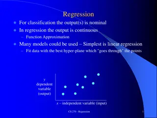
Elastic Net regularization overcomes the limitations of Lasso and Ridge regression in handling biological data with correlated variables. By combining the strengths of L1 and L2 penalties, Elastic Net can automatically select variables, encourage group effects, and offer better prediction accuracy. This comprehensive approach provides a balance between sparsity and grouping, making it a powerful tool in machine learning models.

Download Presentation

Please find below an Image/Link to download the presentation.
The content on the website is provided AS IS for your information and personal use only. It may not be sold, licensed, or shared on other websites without obtaining consent from the author.If you encounter any issues during the download, it is possible that the publisher has removed the file from their server.
You are allowed to download the files provided on this website for personal or commercial use, subject to the condition that they are used lawfully. All files are the property of their respective owners.
The content on the website is provided AS IS for your information and personal use only. It may not be sold, licensed, or shared on other websites without obtaining consent from the author.
E N D
Presentation Transcript
Penalized Regression, Part 3 BMTRY 790: Machine Learning
Limitations of the Lasso Many biological data we encounter have p > n Gene expression, clinical data warehouse data Variables in such data also are often correlated (grouped variables) lasso fails to do grouped selection. An ideal selection method should be able to Remove all unimportant variables Automatically include whole groups in a model once one member of the group is included It seems like a some combination of ridge and lasso regression might work .
Elastic Net Combines the ridge and lasso penalties in the objective function (Zou and Hastie, 2005) ( i i = ) 2 ( ) n p p p = + + 2 j M Y X 0 2 1 i ij j j = = = 1 1 1 j j j The L1(lasso) part of the penalty generates a sparse model. The L2(ridge) quadratic part of the penalty Removes the limitation on the number of selected variables Encourages grouping effect Stabilizes the L1regularization path
Elastic Net Regularization Elastic Net penalty function Has singularity at the vertices (sparsity) Has strict convex edges (encourages grouping) Properties Simultaneously does variable selection and continuous shrinkage Can select groups of correlated variables The elastic net often outperforms the lasso in terms of prediction accuracy
Nave Elastic Net 1 2 , , L n n n = = = 2 ij 0; 0 & 1 y x x Initialize i ij = = = 1 1 1 i i i ( ) 2 ( ) ( ) n p p p = = + + 2 j , , M L Y X 1 2 2 1 i ij j j i i = = = = 1 1 1 j j j ( ) Then: = argmin If we let then we can rewrite the solution as 1 2 + ( 1 i j = = = 2 ) 2 n p = argmin y x i ij j 1 ( ) p p + 2 j subjectto: 1 t j = = 1 1 j j The impact of :
Geometry of Elastic Net Elastic Net Penalty: ( ) p p = + 2 j p 2 1 j = = 1 1 j j ( ) p p = + 2 j 1 j = = 1 1 j j = 2 + 2 1 Singularities at the vertexes (necessary for sparsity) Strict convex edges. The strength of convexity varies with (grouping).
Nave Elastic Net Solution ( ) ( ) X 1: Given data , and some , , define a "artificial dataset" Lemma y 1 2 ( ) * * X , where y X y 0 = = * * X y 1 + ( ) ( ) n p + n p + 1 p I 1 2 2 = = + . Then we can rewrite our elastic net criterion as ( ( , L * Let & 1 1 2 + 1 2 ) ( ) 2 n p + p p = + * * i * ij * j * j , L y x = = = 1 1 1 i j j ) = * * argmin * enetniave = * Then 1 + 1 2
Grouped Variables Grouped variables occur when predictors within the X matrix are highly correlated Microarray data (genes in the same pathway are likely grouped) Environmental contaminant data from similar sources Extreme case: Xi== Xj Ideally regression method identifies these variables as a group and assigns similar coefficient values (assuming scaled and centered) Simulations have shown Lasso performs poorly when predictors in X are highly collinear Ridge can handle collinearity BUT not variable selection
Elastic Net For Grouping X 2: Given predictor matrix where j for , 1,2,..., Lemma X X i j p n p = i j ( ) ( ) ( ) If a is strictly convex then 0 p i i p = * ( ) If b , then 0 and isa minimizerof p j j = 1 j ( ) 2 ( ) n p = + argmin whe re y x p i ij j = = 1 1 i j * k if and k k = k i k j ( )( ) )( 1 = + = * k * i * j if if s i j ( ) + * i * j s for any 0,1 s
Corrected Elastic Net Solution Assume have data (y, X) and ( 1, 2) and augmented data (y*, X*) Recall the na ve solution ( * 1 1 i j ) 2 n p + p p = + = = + * * i * ij * j * j * argmin ; and 1 y x 1 2 + = = = 1 1 j 2 = * enetniave whichyields: 1 + 1 2 To avoid the double penalty, Zou and Hastie apply a correction = + * enet 1 2 ( ) = + enetniave 1 2
Computing Elastic Net Solution Recall, the full Lasso path could be calculated using a modified version of the least angle regression (LAR) algorithm Sequentially add predictors most correlated with residuals LAR: Once a variable is in the active set, it remains in the active set Modified LAR (i.e. lasso path): Variables that cross 0 removed from active set LAR-EN algorithm imposes an additional constraint Apply modified LAR algorithm but based on a fixed quadratic penalty term, 2
LARS-EN Algorithm LARS-EN algorithm: (1) Initialize 2and model: with empty active set A0 and = 0 = r y y (2) Find the most correlated with r and update the active set to 1j X = A X 1 j 1 ols j X (3) Move towards , until another covariate has the same correlation with r that does. Update active set to 1j X 1 ( 1 2 X j 2j 1 1 = , A X X 2 j j 2 ) ( ) (4) Update r and move along towards the joint OLS direction for until a third covariate is as correlated with r as .Update active set to 3j , , X X j j j j ( ) 1 = 2 , , A X X X , X X 3 j j j j j 1 2 3 1 2 (4a) If a non-zero coefficient reaches 0, remove it from the active set and recalculate the current joint OLS direction (5) Continue until all p covariates have been added to the model
Elastic Net vs. Lasso Consider data with 2 hidden factors z1and z2 ( ) ( ) ~ 0,20 ~ 0,20 z U z U 1 2 With response y where y = z1+ 0.1z2+ We observe predictors x z x z = + ( ~ N(0, 1/16)) = + = = + + = = + + x x z z x x z z 1 1 1 2 1 2 3 1 3 4 2 4 5 2 5 6 2 6 Fit a model on (X, y) Ideally, an oracle model identifies x1, x2, and x3as important
Lasso and Elastic Net Paths Elastic Net Path for 2 = 1 Lasso Path
Tuning Elastic Net Models As with ridge and lasso regression, we need to tune our models for an appropriate choice of penalty parameter However, in elastic net we have two penalty parameters to consider We can think about parameters we need to tune in several ways Tune based on ( 1, 2) Based on 2 and the L1-norm (i.e. ) Second parameter: L1-norm = t Or second parameter: fraction of L1-norm = s The second choice is common Alternatively based on 2 and the number of maximum number of steps This is a good choice if p > nand want to limit the number of predictors considered p j = 1 j
Tuning Elastic Net Models We can choose any of the approaches and use a cross-validation approach Ridge we used a generalized cross validation approach (like leave one out) Lasso we used K-fold cross validation (common choices for K are 5 and 10) BUT we need to consider that we have a 2-D surface to optimize Could conduct a grid search with K-fold cross validation Select a set of fixed 2 (generally something like c(0, 0.01, 0.1, 1, 10, 100)) Then apply K-fold cross validation for each 2 based on a sequence of parameter 2 Select the combination of 2 and parameter 2 that yield the smallest CV error
Software Packages There are (at least) 2 packages in R that can fit glmnet, elasticnet The elasticnet package is based on the lars package we used for fitting lasso models Has build in cross-validation function Set 2 and then examine choice of either (a) fraction of L1-norm (b) maximum number of steps However, the glmnet package can fit an elastic net model However, appears to be based on the na ve elastic net approach
Body Fat Example Recall our regression model > summary(mod13) Call: lm(formula = PBF ~ ., data = bodyfat2) Estimate Std. Error t value Pr(>|t|) (Int) 0.000 3.241e-02 0.000 1.00000 Age 0.0935 4.871e-02 1.919 0.05618 . Wt -0.3106 1.880e-01 -1.652 0.09978 . Ht -0.0305 4.202e-02 -0.725 0.46925 Neck -0.1367 6.753e-02 -2.024 0.04405 * Chest -0.0240 9.988e-02 -0.241 0.81000 Abd 1.2302 1.114e-01 11.044 < 2e-16 *** Hip -0.1777 1.249e-01 -1.422 0.15622 Thigh 0.1481 9.056e-02 1.636 0.10326 Knee 0.0044 6.974e-02 0.063 0.94970 Ankle 0.0352 4.485e-02 0.786 0.43285 Bicep 0.0656 6.178e-02 1.061 0.28966 Arm 0.1091 4.808e-02 2.270 0.02410 * Wrist -0.1808 5.968e-02 -3.030 0.00272 ** Residual standard error: 4.28 on 230 degrees of freedom Multiple R-squared: 0.7444, Adjusted R-squared: 0.73 F-statistic: 51.54 on 13 and 230 DF, p-value: < 2.2e-16
Body Fat Example library(elasticnet) ### First conducting 10-fold CV to select our tuning parmaters ### par(mfrow=c(2,3)) set.seed(3210) menet0<-cv.enet(x=bodyfat2[,2:14], y=bodyfat2[,1], s=seq(0,1,length=100), lambda=0, mode="fraction") set.seed(3210) menet001<-cv.enet(x=bodyfat2[,2:14], y=bodyfat2[,1], s=seq(0,1,length=100), lambda=0.01, mode="fraction") set.seed(3210) menet01<-cv.enet(x=bodyfat2[,2:14], y=bodyfat2[,1], K=10, s=seq(0,1,length=100), lambda=0.1, mode="fraction") set.seed(3210) menet1<-cv.enet(x=bodyfat2[,2:14], y=bodyfat2[,1], K=10, s=seq(0,1,length=100), lambda=1, mode="fraction") set.seed(3210) menet10<-cv.enet(x=bodyfat2[,2:14], y=bodyfat2[,1], K=10, s=seq(0,1,length=100), lambda=10, mode="fraction") set.seed(3210) menet100<-cv.enet(x=bodyfat2[,2:14], y=bodyfat2[,1], K=10, s=seq(0,1,length=100), lambda=100, mode="fraction")
Body Fat Example Let s look at one of the models >names(menet01) [1] "s" "cv" "cv.error" > menet01$s [1] 0.00000000 0.01010101 0.02020202 0.03030303 0.04040404 0.05050505 [97] 0.96969697 0.97979798 0.98989899 1.00000000 > menet01$cv [1] 0.9979108 0.9561537 0.9157728 0.8767680 0.8391396 0.8028873 0.7680113 [99] 0.2876542 0.2879505 > menet01$cv.error [1] 0.08570741 0.08403771 0.08243508 0.08088946 0.07939103 0.07793024 [97] 0.02713857 0.02699345 0.02684893 0.02670769
Body Fat Example ### Looking at minimum cv error for each choice of lambda_2 > min(menet0$cv) [1] 0.2864688 > min(menet001$cv) [1] 0.2914921 > min(menet01$cv) [1] 0.3226485 > min(menet1$cv) [1] 0.4163464 > min(menet10$cv) [1] 0.4479238 > min(menet100$cv) [1] 0.4522492
Body Fat Example ### Selecting the fraction of L1-Norm from the model with the smallest cv.error > fracL1<-menet0$s[which(menet0$cv==min(menet0$cv))] > fracL1 0.8787879 ### fitting a model with our choice of lambda_2 > mod.enet<-enet(x=bodyfat2[,2:14], y=bodyfat2[,1], lambda=0) > plot(mod.enet, use.color=T, main="Body Fat Example") > abline(v=fracL1, lty=2, col=2, lwd=2)
Body Fat Example ### extracting the model based on the selected lambda_2 and fraction of L1 > predict(mod.enet, s=fracL1, type= coefficients ) $s [1] 0.8787879 $fraction 0 0.8787879 $mode [1] "fraction" $coefficients Age Wt Ht Neck Chest Abd 0.09124856 -0.24657606 -0.03803826 -0.12674220 0.00000000 1.15383642 Hip Thigh Knee Ankle Bicep Arm -0.13079181 0.10911306 0.00000000 0.01882265 0.04902691 0.09836029 Wrist -0.17520256
Summary of Common Penalized Regression Penalized regression model take the general form ( 1 i j = ) 2 ( ) q n p p = + 0 M y x q q i ij j j = = 1 1 j Most common choices for these models include Ridge: ( ) 2 M = ( ) 1 i M ( ) 2 2 n p p + 2 j y x 2 i ij j ) = = = 1 ( 1 1 i j j Lasso: n p p = + y x 1 i ij j j = = = 1 1 1 j j ( ) 2 ( ) n p p p Elastic Net: = + + 2 j M y x 1 2 i ij j j = = = = 1 1 1 1 i j j j None are oracle methods BUT they have useful properties
Summary of Common Penalized Regression All improve prediction via bias-variance trade-off Recall OLS solution is BLUE (among unbiased solutions) Penalized approaches increase bias but generally reduce variance In all of these approaches, solutions are not scale invariant Scale and center variables (and often outcome) before fitting Only exception are categorical responses Shrinkage/penalty parameters must also be tuned before selecting final model Generalized cross validation (relevant only to ridge regression) K-fold cross validation
Adaptations to Penalized Regression Models Methods designed to achieve oracle properties Choose Lq where 0 < q < 1 Constraint region no longer convex so harder to solve Smoothly Clipped Absolute Deviation (SCAD) penalty (Fan and Li 2001) Use of weighted sum of predictors in penalty Weighted and adaptive Lasso (Zou 2006; Zhang and Lu 2007) ( ) 1 j j j p w = = n Nonnegative garrote ( ) n p p + ols j min subject to 0 y x c c c 1,...c c i ij j j j = = = 1 1 1 i j j p
Adaptations to Penalized Regression Models Methods for correlated predictors Adaptive Elastic Net ( ) 2 ( ) n p n n = + + + 2 j aenet 1 argmin y x w 2 2 1 i ij j j j = = = = 1 1 1 1 i j j j ( ) = forsome constant 0 w j j Group variable selection Grouped Lasso (and adaptive group lasso) ( ) 2 n p n = + glasso argmin y x p i ij j j j = = = 1 1 1 i j j supnorm penalty ( ) p = maxj j
Next Time Finalize our discussion of linear regression model fitting strategies Moving to classification (i.e. non-continuous outcome) Start our discussion of linear classifiers