Performance Evaluation of Manufacturing Systems
Dive into the world of manufacturing systems with a focus on performance evaluation. Learn about discrete event systems, system basics, input-output modeling, static and dynamic systems, and more. Explore key concepts, theories, and practical examples to enhance your knowledge in this field.

Download Presentation

Please find below an Image/Link to download the presentation.
The content on the website is provided AS IS for your information and personal use only. It may not be sold, licensed, or shared on other websites without obtaining consent from the author. If you encounter any issues during the download, it is possible that the publisher has removed the file from their server.
You are allowed to download the files provided on this website for personal or commercial use, subject to the condition that they are used lawfully. All files are the property of their respective owners.
The content on the website is provided AS IS for your information and personal use only. It may not be sold, licensed, or shared on other websites without obtaining consent from the author.
E N D
Presentation Transcript
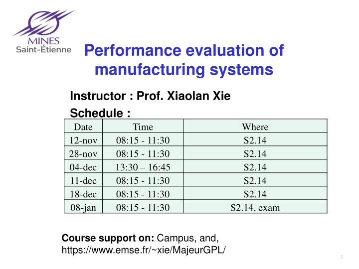
Performance evaluation of manufacturing systems Instructor : Prof. Xiaolan Xie Schedule : Date Time 12-nov 08:15 - 11:30 28-nov 08:15 - 11:30 04-dec 13:30 16:45 11-dec 08:15 - 11:30 18-dec 08:15 - 11:30 08-jan 08:15 - 11:30 Where S2.14 S2.14 S2.14 S2.14 S2.14 S2.14, exam Course support on: Campus, and, https://www.emse.fr/~xie/MajeurGPL/ 1
Chapter I Introduction to discrete event systems Learning objectives : Introduce fundamental concepts of system theory Understand features of event-driven dynamic systems Textbook : C. Cassandras and S. Lafortune, Introduction to Discrete Event Systems, Springer, 2007 2
Plan System basics Discrete-event system by an example of a queueing system Discrete event systems 3
System basics 4 4
The concept of system System: A combination of components that act together to perform a function not possible with any of the individual parts (IEEE) Salient features : Interacting components Function the system is supposed to perform 5
The Input-Output Modeling process Define a set of measurable variables Select a subset of variables that can be changed over time (Input variables) Select another set of variables directly measurable (Output variables, responses, stimulus) Derive the Input-Output relation Output Input y(t) = g(u, t) u(t) SYSTEM MODEL 6
The Input-Output Modeling process Example 1 : An electric circuit with two resistances r and R r y(t)/u(t)= R/(r+R) R u(t) y(t) Example 2 : An electric circuit with a resistance R and a capacitor (condensateur) C u(t) = vR(t) + y(t) vR(t) = iR i=C.dy(t)/dt R C u(t) y(t) Y(s)/U(s) = 1/(1+CRs) 7
Static and dynamic systems Static systems : Output y(t) independent of the past values of the input u( ), for < t. The IO relation is a function : y(t) = g(u(t)) Dynamic systems : Output y(t) depends on past values of the input u( ), for < t. Memory of the input history is needed to determine y(t) The IO relation is a differential equation. 8
Static and dynamic systems r Static R + ( ) y K ( ) u K = R r R u(t) y(t) y(K) depends only on u(K) Dynamic R Case u(t) = K & y(0) = K: y(K) = K Case u(t) = K & y(0) = 0 : y(K) = K Ke-K/RC Case u(t) = t & y(0) = 0 : y(K) = K (1-e-K/R)/RC C u(t) y(t) y(K) depends on past u(t) and y(0) 9
The concept of state Definition : The state of a system at time t0 is the information required at t0 such that the output y(t), for all t t0 is uniquely determined from this information and from u(t), t t0. The state is generally a vector of state variables x(t). 10
System dynamics State equation : The set of equations required to specify the state x(t) for all t t0, given x(t0) and the function u(t), t t0. ( ) ( ) ( ) ( , , t t t t = x f x u ) ( ) t = x x , 0 State space : The state space of a system is a set of all possible values that the state may take. Output equation : ( ) t y ( ) ( ) t ( ) t t = g x u , , 11
System dynamics : sample path x(t) x0 t 12
Discrete system The system is observed at regular intervals at time t = n for all constant elementary period . ( ( ) ) += = x f x u x x , , 1 0 0 n n n n = y g x u , n n n n x0 xn t 13
State of the system : x(t) = number of customers in the system Random customer arrivals Random service times FIFO service Server Customer arrivals Queue Customer departures 15
System dynamic The state of the system remains unchanged except at the following instants (events) arrival times t of customers where x(t+0) = x(t 0) +1 departure times t of customers where x(t+0) = x(t 0) 1 Sample path x(t) 16
The concept of event An event occurs instantaneously and causes transitions from one discrete state to another An event can be a specific action taken (press a button) a spontaneous occurrence dictated by nature (failures) sudden fulfillment of some conditions (buffer full). Notation : e = event, E = set of event. Queueing system: E = {a, d} with a = arrival, d = departure 18
Time-driven and event-driven systems Time-driven systems Continuous time systems Discrete systems (driven by regular clock ticks) State transitions are synchronized by the clock Event-driven systems State changes at various time instants (may not known in advance) with some event e announcing that it is occurring State transitions as a result of combining asynchronous and concurrent event processes. 19
Characteristics of discrete event systems Definition. A Discrete Event Systems (DES) is a discrete-state, event-driven system, that is, its state evolution depends entirely on the occurrence of asynchronous discrete events over time. Essential defining elements: E : a discrete-event set X : a discrete state space 20
Two Points of Views Untimed models (logical behavior) event sequence {e1, e2, ...} without information about the occurrence times. Sample path: sequence of states resulting from {s1, s2, ...} Timed models (quantitative behavior) timed event sequence {(e1, t1), (e2, t2), ...}. Sample path : the entire sample path over time. Also called a realization. e1 e2 e3 e4 e5 e1 e2 e3 e4 e5 s1 s2 s3 s4 s5 s6 t1 t2 t3 t4 t5 21
A manufacturing system 2 1 part departures part arrivals A two-machine transfer line with an intermediate buffer of capacity 3. Essential defining elements: E = {a, d1, d2} X = {(x1, x2) : x1 0, x2 {0, 1, 2, 3, B}} 22
System classifications Static vs dynamic systems Time-varying vs time-invariant systems Linear vs nonlinear systems continuous-state vs discrete state systems time-drived vs event-driven systems deterministic vs stochastic systems discrete-time vs continuous-time systems 23
Goals of system theory Modeling and analysis Design and synthesis Control Performance evaluation Optimization 24
Untimed models Model Goal features Formal language (lowest level model) Represent all possible event sequence L = { , f, fr, frf, frfr, } = no event f =machine failure r = repair State-transition representation Regular language L = (fr)*( +f) With repetition (*) union (+) concatenation (.) Finite state automata (low-level model) f up down r Petri nets (high-level model) Compact representation + better explanability up f 3 machines initially up down r 25