Poisson Regression Model with Age, Period, and Area Descriptors

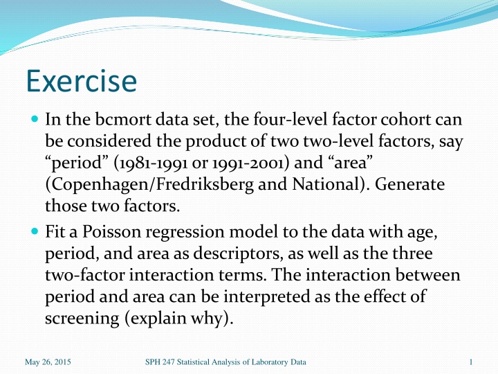
The four-level factor cohort in the bcmort data set can be viewed as a combination of two two-level factors - period (1981-1991 or 1991-2001) and area (Copenhagen/Frederiksberg and National). This exercise involves generating these two factors, fitting a Poisson regression model to the data with age, period, and area as descriptors, along with the three two-factor interaction terms. The interaction between period and area is interpreted as the effect of screening. The model results, including coefficients and significance levels, are presented for the specified descriptors and interactions.

• Poisson Regression
• bcmort Data Set
• Factor Analysis
• Interaction Effects
• Statistical Analysis

car_la Follow

Uploaded on Feb 18, 2025 | 0 Views

Download Presentation

Please find below an Image/Link to download the presentation.

The content on the website is provided AS IS for your information and personal use only. It may not be sold, licensed, or shared on other websites without obtaining consent from the author.If you encounter any issues during the download, it is possible that the publisher has removed the file from their server.

You are allowed to download the files provided on this website for personal or commercial use, subject to the condition that they are used lawfully. All files are the property of their respective owners.

The content on the website is provided AS IS for your information and personal use only. It may not be sold, licensed, or shared on other websites without obtaining consent from the author.

Presentation Transcript

1. Exercise In the bcmortdata set, the four-level factor cohort can be considered the product of two two-level factors, say period (1981-1991 or 1991-2001) and area (Copenhagen/Fredriksberg and National). Generate those two factors. Fit a Poisson regression model to the data with age, period, and area as descriptors, as well as the three two-factor interaction terms. The interaction between period and area can be interpreted as the effect of screening (explain why). May 26, 2015 SPH 247 Statistical Analysis of Laboratory Data 1

2. > library(ISwR) > data(bcmort) > summary(bcmort) age cohort bc.deaths p.yr 50-54:4 Study gr. :6 Min. : 9.0 Min. : 25600 55-59:4 Nat.ctr. :6 1st Qu.: 51.0 1st Qu.: 86434 60-64:4 Hist.ctr. :6 Median :104.0 Median : 169261 65-69:4 Hist.nat.ctr.:6 Mean :213.2 Mean : 396520 70-74:4 3rd Qu.:436.2 3rd Qu.: 781897 75-79:4 Max. :545.0 Max. :1067778 > class(bcmort$cohort) [1] "factor" > dim(bcmort) [1] 24 4 > bcmort$cohort [1] Study gr. Study gr. Study gr. Study gr. Study gr. Study gr. Nat.ctr. [8] Nat.ctr. Nat.ctr. Nat.ctr. Nat.ctr. Nat.ctr. Hist.ctr. Hist.ctr. [15] Hist.ctr. Hist.ctr. Hist.ctr. Hist.ctr. Hist.nat.ctr. Hist.nat.ctr. Hist.nat.ctr. [22] Hist.nat.ctr. Hist.nat.ctr. Hist.nat.ctr. Levels: Study gr. Nat.ctr. Hist.ctr. Hist.nat.ctr. > area <- factor(gl(2,6,24,c("Local","National"))) > period <- factor(gl(2,12,24,c("1990s","1980s"))) May 26, 2015 SPH 247 Statistical Analysis of Laboratory Data 2

3. > data.frame(bcmort$cohort,area,period) bcmort.cohort area period 1 Study gr. Local 1990s 2 Study gr. Local 1990s 3 Study gr. Local 1990s 4 Study gr. Local 1990s 5 Study gr. Local 1990s 6 Study gr. Local 1990s 7 Nat.ctr. National 1990s 8 Nat.ctr. National 1990s 9 Nat.ctr. National 1990s 10 Nat.ctr. National 1990s 11 Nat.ctr. National 1990s 12 Nat.ctr. National 1990s 13 Hist.ctr. Local 1980s 14 Hist.ctr. Local 1980s 15 Hist.ctr. Local 1980s 16 Hist.ctr. Local 1980s 17 Hist.ctr. Local 1980s 18 Hist.ctr. Local 1980s 19 Hist.nat.ctr. National 1980s 20 Hist.nat.ctr. National 1980s 21 Hist.nat.ctr. National 1980s 22 Hist.nat.ctr. National 1980s 23 Hist.nat.ctr. National 1980s 24 Hist.nat.ctr. National 1980s May 26, 2015 SPH 247 Statistical Analysis of Laboratory Data 3

4. > drop1(glm(bc.deaths ~ age+period+area+age:period+age:area+period:area+offset(log(p.yr)) ,family=poisson),test="Chisq") Single term deletions Model: bc.deaths ~ age + period + area + age:period + age:area + period:area + offset(log(p.yr)) Df Deviance AIC LRT Pr(Chi) <none> 5.458 202.405 age:period 5 34.792 221.739 29.334 1.994e-05 *** age:area 5 17.279 204.226 11.821 0.0373179 * period:area 1 16.775 211.722 11.317 0.0007678 *** --- Signif. codes: 0 *** 0.001 ** 0.01 * 0.05 . 0.1 1 May 26, 2015 SPH 247 Statistical Analysis of Laboratory Data 4

5. > summary(glm(bc.deaths ~ age+period+area+age:period+age:area+period:area+offset(log(p.yr)), family=poisson),test="Chisq") Coefficients: Estimate Std. Error z value Pr(>|z|) (Intercept) -8.71065 0.20674 -42.133 < 2e-16 *** age55-59 0.59227 0.23373 2.534 0.011277 * age60-64 1.08881 0.22321 4.878 1.07e-06 *** age65-69 1.24619 0.21945 5.679 1.36e-08 *** age70-74 1.62200 0.21709 7.472 7.93e-14 *** age75-79 1.93431 0.23583 8.202 2.36e-16 *** period1980s 0.76507 0.15539 4.924 8.50e-07 *** areaNational -0.36892 0.20220 -1.825 0.068070 . age55-59:period1980s -0.34415 0.14996 -2.295 0.021735 * age60-64:period1980s -0.55380 0.14786 -3.746 0.000180 *** age65-69:period1980s -0.58432 0.14731 -3.967 7.29e-05 *** age70-74:period1980s -0.65739 0.14776 -4.449 8.62e-06 *** age75-79:period1980s -0.56839 0.16360 -3.474 0.000512 *** age55-59:areaNational 0.69382 0.22708 3.055 0.002248 ** age60-64:areaNational 0.52311 0.21633 2.418 0.015600 * age65-69:areaNational 0.49641 0.21251 2.336 0.019492 * age70-74:areaNational 0.38044 0.21047 1.808 0.070675 . age75-79:areaNational 0.33547 0.22865 1.467 0.142325 period1980s:areaNational -0.29262 0.08796 -3.327 0.000879 *** > tapply(bc.deaths/p.yr,list(area,period),mean)*100000 1990s 1980s Local 57.42036 74.18913 National 61.76304 57.55497 May 26, 2015 SPH 247 Statistical Analysis of Laboratory Data 5

6. Exercise 2 Use the elastic net to develop predictors for AD vs. NDC. Try repeated cross-validation runs and compare the plots. What happens if we use = 0.3 or 0.7 instead of 0.5? Why would we run into difficulties if we used cross- validated logistic regression? Repeat the analysis for AD vs. OD. May 26, 2015 SPH 247 Statistical Analysis of Laboratory Data 6

7. > library(glmnet) > dim(ad.data) [1] 104 125 > diagnosis <- ad.data[,1] > summary(diagnosis) AD NDC OD 33 30 41 > isub <- diagnosis != "NDC" > admat.net <- as.matrix(ad.data[isub,-1]) > diag.net <- droplevels(diagnosis[isub]) > summary(diag.net) AD OD 33 41 > ad.cv <- cv.glmnet(admat.net,diag.net,family="binomial") > lmin <- ad.cv$lambda.min > l1se <- ad.cv$lambda.1se > lmin [1] 0.01028176 > l1se [1] 0.0630879 May 26, 2015 SPH 247 Statistical Analysis of Laboratory Data 7

8. > ad.net <- glmnet(admat.net,diag.net,family="binomial") > predict(ad.net,s=lmin,type="nonzero") X1 1 1 2 8 3 10 4 12 5 20 6 22 25 113 26 117 27 118 > predict(ad.net,s=l1se,type="nonzero") X1 1 1 2 10 3 12 4 17 5 28 6 32 7 69 8 78 9 93 10 110 11 120 May 26, 2015 SPH 247 Statistical Analysis of Laboratory Data 8

9. > colnames(admat.net)[predict(ad.net,s=l1se,type="nonzero")$X1] [1] "ACE..CD143." "ApoAI" "ApoB" [4] "Apolipoprotein.A1" "Calcitonin" "CD40.Ligand" [7] "IGF.1" "IL.18" "MIF" [10] "Prostate.Specific.Antigen..Free" "Stem.Cell.Factor" > plot(cv.glmnet(admat.net,diag.net,family="binomial",type="class")) > plot(cv.glmnet(admat.net,diag.net,family="binomial")) May 26, 2015 SPH 247 Statistical Analysis of Laboratory Data 9

10. May 26, 2015 SPH 247 Statistical Analysis of Laboratory Data 10

11. May 26, 2015 SPH 247 Statistical Analysis of Laboratory Data 11

12. May 26, 2015 SPH 247 Statistical Analysis of Laboratory Data 12

13. May 26, 2015 SPH 247 Statistical Analysis of Laboratory Data 13

14. May 26, 2015 SPH 247 Statistical Analysis of Laboratory Data 14

15. May 26, 2015 SPH 247 Statistical Analysis of Laboratory Data 15

16. > predict(ad.net.5,s=l1se,type="nonzero") X1 1 1 2 4 3 8 4 10 5 12 30 113 31 117 32 118 33 120 > colnames(admat.net)[predict(ad.net.5,s=l1se,type="nonzero")$X1] [1] "ACE..CD143." "Agouti.Related.Protein..AgRP." [3] "Angiopoietin.2..ANG.2." "ApoAI" [5] "ApoB" "ApoE" [7] "ApoH" "Apolipoprotein.A1" [9] "Apolipoprotein.CIII" "ASP" [11] "B.Lymphocyte.Chemoattractant..BLC." "Betacellulin" [13] "Calcitonin" "CD40.Ligand" [15] "Cortisol" "Creatine.Kinase.MB" [17] "EGF.R" "Ferritin" [19] "FSH" "HCC.4" [21] "IGF.1" "IL.13" [23] "IL.18" "MCP.3" [25] "MDC" "MIF" [27] "MIP.1.alpha" "Prostate.Specific.Antigen..Free" [29] "Pulmonary.and.Activation.Regulated.Chemokine..PARC." "PYY" [31] "SGOT" "SHBG" [33] "Stem.Cell.Factor" May 26, 2015 SPH 247 Statistical Analysis of Laboratory Data 16

17. > plot(cv.glmnet(admat.net,diag.net,family="binomial",type="class",alpha=0.5)) > preds.5 <- predict(ad.net.5,s=l1se,newx=admat.net,type="class") > table(preds.5,diag.net) diag.net preds AD OD AD 31 0 OD 2 41 > preds <- predict(ad.net,s=l1se,newx=admat.net,type="class") > table(preds,diag.net) diag.net preds AD OD AD 30 0 OD 3 41 Plots show minimum cross-validated error is between 10% and 20%. If we predict to the whole data set using a model fitted from the whole data set, the apparent error is under 5%. The former estimate is the more realistic. Even better would be to do nested CV. If we predict at lambda = lmin, the apparent error rate is near 0. May 26, 2015 SPH 247 Statistical Analysis of Laboratory Data 17

18. May 26, 2015 SPH 247 Statistical Analysis of Laboratory Data 18