Pole Expansion and Proof of Mittag-Leffler Theorem
Dive into the Pole Expansion of a Function via the Mittag-Leffler Theorem with detailed proofs, contour integrals, residue analysis, and extended theorem variations. Explore series expansion techniques and pole analysis in complex functions.

Download Presentation

Please find below an Image/Link to download the presentation.
The content on the website is provided AS IS for your information and personal use only. It may not be sold, licensed, or shared on other websites without obtaining consent from the author.If you encounter any issues during the download, it is possible that the publisher has removed the file from their server.
You are allowed to download the files provided on this website for personal or commercial use, subject to the condition that they are used lawfully. All files are the property of their respective owners.
The content on the website is provided AS IS for your information and personal use only. It may not be sold, licensed, or shared on other websites without obtaining consent from the author.
E N D
Presentation Transcript
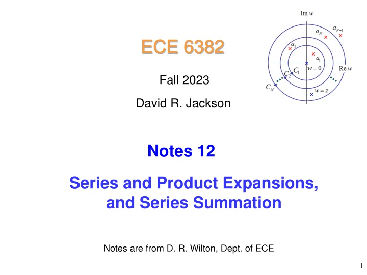
ECE 6382 Fall 2023 David R. Jackson Notes 12 Series and Product Expansions, and Series Summation Notes are from D. R. Wilton, Dept. of ECE 1
Pole Expansion of a Function (Mittag-Leffler Theorem) Mittag-Leffler Theorem Assumptions: An extension would be pairs of poles occurring at increasing distance from the origin. = = has simple poles at has residue , independent of , on circles g through any of them and such that where ( ) ( ) ( ) f z N poles, not passin , 1,2, , 0 f z f z z a n a a a 1 2 3 n n = = at , 1,2, b z a n n N of radius that enclose R M C R N N N N Then Note: b b a If the sum is finite, this becomes a partial fraction expansion. = + + ( ) f z (0) f n n z a = 1 n n n This is an expansion in terms of residues! Note: Each of the two individual series in the sum may not converge. Note that a pole at the origin is not allowed! But we can always shift using z z - z0. Or we can add a term to cancel a pole that appears at the origin. Magnus Gustaf (G sta) Mittag-Leffler 2
Proof of Mittag-Leffler Theorem For , consider the sequence of contour integrals: z a n 1 = ( ) ( ) I F w dw F w residues N 2 i C N where ( ) w f ( ) w F Imw ( ) w w z a a + 1 N ( ) N = Res ( ) lim w ( ) F w w w F w p p 2 a w p 1 R 1a (0) z ( ) f z z f ( ) 0 = Residue F w = 0 Rew C C 1 2 ( ) = Residue F z C = w z N b ( ) F a = Residue n ( ) n a a z n n 3
Proof of Mittag-Leffler Theorem N 1 ( ) ( w w (0) z ( ) f z z f w dw z f b = + + I n (from the residue theorem) N 2 ) ( ) i a a z = 1 n n n C N Imw = i But we also have for on w R e C N N f R e a i ( R ) R d 2 a + 1 ( ( ) 1 1 N f w dw w w N N z N I N 2 ) 2 ( ) i z R 2 a N N 0 C N 2 R 1a M R R 1 N 0 w = 0 Rew N 2 ( ) z C C 1 N N 2 C = w z N Taking the limit as N , we have (0) z ( ) f z z f b + + = 0 n N I 0 ( ) a a z = 1 n n n 4
Proof of Mittag-Leffler Theorem (0) z ( ) f z z f b + + = 0 n Imw ( ) a a z = 1 n n n a a + 1 N N Multiply by z, and solve for f(z): 2 a 1a zb = ( ) f z (0) f n Rew ( ) a a z C C = 1 n 1 n n 2 C N Then use a partial fraction expansion: b b a b b a = = + + ( ) f z (0) (0) f f n n n n a z z a = = 1 1 n n n n n n (proof complete) 5
Extended Form of the Mittag-Leffler Theorem Extended Mitag-Leffler Theorem Asumptions: = = has simple poles at has residue where ( ) ( ) f z , 1,2, , 0 f z z a n a a a 1 2 3 n n = = at , 1,2, b z a n n p (for integer ) , independent of , on circles that enclose poles, n ot passing through any of them and such that of radius ( ) f z M z p N C R N N N R N N Then consideration of the integral 1 ( ) ( f w dw w z = I N + 1 p 2 ) i w C N leads to the this expansion: + + ( ) p 1 1 p p p n (0) / a z f b z a (0) = + + + + ( ) f z (0) f zf n ! p z = 1 n n Note: The first p terms are those of a Taylor series. 6
Example: Pole Expansion of cotz cos sin z z = = = 0, 1, 2, cot z has poles with residues , z n n cos d d z cos cos z z z = = = , lim z lim z 1. 1 . b Hence n n n sin z = Then, since a pole at is not allowed, consider 0 z 1 z = ( ) f z cot , z for which the singularity a a removeable singularity at the origin with a finite limit: t the origin has been removed and which has 1 z cos sin + 1 z cos sin z z z z z z = = lim cot z lim z lim z z sin z 0 0 0 = 2 3 z z 1 2 1 6 + + 1 z z + + 3 5 O ( ) z z 2! 3! = lim z lim z 0 2 4 3 O ( ) z z z 0 0 + z z 3! (The finite limit is actually zero here.) 7
Example: Pole Expansion of cot z(cont.) Figure showing the circles 1 z = = = ( ) f z cot z , 1,2, n a n n Poles at: 1 ( ( ) f w w dw z v = I N 2 ) i w C 4 C = w z N C 2 C 0 u 2 3 Note: 2 In this case it is pairs of poles that are of increasing distance from the origin. 5 2 In this case N is always even. 8
Example: Pole Expansion of cot z(cont.) , independent of , on circles Assumption: ( ) f z M N C N cos sin z z i = = To check that is bounded on use where cot , z C z R e N N (2 1) N = = so that threads between the poles at , and tha t R C z n N N v 2 C ( ( ) ) 4 2 2 ( ( ) ) i = + + w z cos R e cos sin cos cos sin sin R R i i C 2 N N = = 2 cot z i sin R e C 0 N N u 2 ( ( ) ) ( ( ) ) ( ( ) ) ( ( ) ) + cos sin cos cos cosh cosh sin sin sin cos cos cos sinh sinh sin sin R R R R i i R R R R 2 = N N N N 3 2 N N N N ( ( ) ) ( ( ) ) ( ( ) ) ( ( ) ) + + 2 2 2 2 cos sin cos cos cosh cosh sin sin sin cos cos cos sinh sinh sin sin R R R R R R R R 5 = N N N N 2 2 2 2 2 N R R N R ( ( N N ( ( ) ) ) ) 2 2 cosh cosh sin sin sin cos cos cos = N N 2 2 R N N = + = 2 2 2 2 where we've used and in both numerator and denominator. sinh cosh 1 sin cos 1 x x x x 9
Example: Pole Expansion of cot z(cont.) Now if we plot the expression ( ( ) ) ( ( ) ) 2 2 cosh cosh sin sin sin cos cos cos R R R R (2 1) N 2 = = N N cot R z N 2 2 2 N N 2 for , for various values of , it appears that 0 /2 cot 1.18823 N z = so that , independent of cot 1.18823 . z M N |cot z|^2 on circular arcs R_n =(N-1/2)pi/2 1.4 1.2 It isn t necessary that the paths CN be circular; see the next slide. 1 N=1 N=2 N=3 N=4 N=8 |cot z|^2 0.8 0.6 0.4 0.2 0 0 0.5 1 1.5 2 Theta (radians) 10
Example: Pole Expansion of cot z(cont.) Alternatively, we could consider the e xpression on the contours shown below: 2 2 + + + 2 2 2 2 cos( sin( ) ) cos cosh sin cosh x ) 2 cosh sinh sin sinh cos sinh x cos sin cosh cosh sin cos sinh sinh x iy x iy + x y i y i + x y y x x y y x x y y 2 = = = cot z 2 2 2 2 ( 2 = + + 2 tanh cos sin 1 , 2 x x 1 2 y x N 2 2 cosh s inh sin cos x x y y y ( ) = = 2 2 coth coth 2, 2 1 2 y y N 2 2 2 2 y 1 ( ) ( w w f w dw = It is easy to then show that on these also 0 . I C N N N 2 ) i z C N v C 4 coth (x) = w z C cot coth2 z z 2 C cot 1 0 u 2 3 2 5 11 2
Example: Pole Expansion of cot z(cont.) Hence, we have 1 z b b a ( ) = = = = + + , 1,2, n a n n ( ) f z cot (0) n n z f ( ) z a = n n n n 0 b b a b b a = + + + + (0) f n n n n ( ) ( ) z a z a = = 1 1 n n n n n n 1 1 1 1 = + + + + 0 ( ) ( ) z n n z n n = = 1 1 n n 1 1 1 1 = + + + 0 + ( ) ( ) z n n z n n = = 1 1 n n Combining the two series and putting over a common demoninator, 1 z 2 z n This result could be helpful for summing this series in closed form. = + cot z 2 2 2 z = 1 n 12
Other Pole Expansions 1 1 z 2 1 1 z 2 z n z n = = + 2 2 2 2 2 2 sin sinh z z z z = = 1 1 n n ( ) ( ) + + 2 + 1 2 + 1 n n 1 1 = = ( ) ( ) 2 2 cos cosh z z 2 1 2 1 n n = = 0 0 n n + 2 2 z z 2 2 2 2 z z = = tan tanh z z ( ) ( ) 2 2 + + 2 1 2 1 n n = = 0 0 n n + 2 2 z z 2 2 1 z 2 1 z 2 z n z n = + = + cot coth z z + 2 2 2 2 2 2 z z = = 1 1 n n The Mittag-Leffler theorem generalizes the partial fraction representation of a rational function to meromorphic functions that have an infinite number of poles. 13
Infinite Product Expansion of Entire Functions Weierstrass s Factorization Theorem Assumptions: is an entire function has simple zeros at where ( ) ( ) f z f z = = , 1, , z a a n Karl Theodor Wilhelm Weierstrass n 0 a a 1 2 3 f z ( ) ( ) f z , independent of , on circles of radius that do not M N C R N N pass through zer os of and such that ( ) f z R N N Then z (0) (0) z f z = a f ( ) f z (0) 1 f e e n a = 1 n n There exists a generalization to multiple-order zeros (Schaum's Complex Variables , p. 267). 14
Product Expansion Formula Proof: ( ) = Near any simple zero where derivative, , must have the form , ( ) f z ( ) f z . Hence the ( ) g z a z a n n logarithmic = is analytic and non-vanishing at ( ) g z z z 0 f z g z ( ) ( ) f z 1 1 ( ) ( ) g z d dz d dz d dz with residue By the Mittag-Leffler ( ) = = + = + , ln ( ) f z ln ln ( ) z a g z ( ) n z a n = has a simple pole at each point . z a n f z ( ) ( ) f z (0) (0) 1 1 a f f = + + theorem, which, on integrating both sides, yiel , ds z a = 1 n n n ( ) f z z z a ( ) ( ) f z ( ) (0) (0) ( 0 f z f f f z = = = + + n . ln ( ) f z ln (0) f ln ln dz z ) a a = 1 n n n 0 Upon exponentiating, we obtain the desired result , z z z z z (0) (0) (0) (0) (0) (0) z f z f z f + z ln 1 ln 1 a a a = = = a a f f f ( ) (0) (0 ) (0) 1 f z f e e f e e e f e e n n n = 1 n n n a = = 1 1 n n n 15
Useful Product Expansions 2 2 z z = = + sin 1 sinh 1 z z z z 2 2 2 2 n n = = 1 1 n n 2 2 4 4 z z = = + cos 1 cosh 1 z z ( ) ( ) 2 2 2 2 2 1 2 1 n n = = 1 1 n n ( ) ( ) 2 2 + z z 1 1 2 2 2 2 n n = = tan tanh z z z z = = 2 2 1 1 n n 4 4 + z z 1 1 2 2 ( ) ( ) 2 2 2 1 2 1 n n Product expansions generalize the factorization of the numerator and denominator polynomials of a rational function into products of their roots. 16
The Argument Principle First consider the following integral: z f z 1 ( ) ( ) f z 1 d dz = ln ( ) f z dz I dz C 2 2 i i C C log derivative ( ) M = ( ) f z z z where 0z 0 (The integer M can be either positive or negative.) pole zero 1 1 1 d dz d dz M ( ) ( ) M = = = = ln ln I z z dz M z z dz dz M 0 0 2 2 2 i i i z z 0 C C C So we have Simple pole with residue 1 = I M Note: The path C does not have to be a circle. 17
The Argument Principle (cont.) Next, we consider extending this to an arbitrary function that is analytic inside a region except for poles of finite order. The function may also have zeros. f z 1 ( ) ( ) f z 1 d dz = ln ( ) f z dz I dz C 2 2 i i C C 3a Zeros or poles 4 a 2 a The integrand in analytic everywhere except where f has a zero or a pole. 1a We can shrink the path C down to small paths that go around each zero and pole. 18
The Argument Principle (cont.) 1 d dz = ln ( ) f z dz I 2 i n C C n 3 C 3a 4 Assume that f(z) has a pole or a zero of order (multiplicity) Mn at z = an. Zeros or poles 4 a C 2 a 1 0: 0: - M M M M zero of order n n 1a C 2 pole of order n n Taylor series for g(z) (valid till we hit the closest singularity to an) Near we can write a n ( ) ( . ( ) ( ) ( ) ) 2 M M = + + + = ( ) z ( ) g z f z a b b z a b z a z a n n 0 1 2 n n n n = where is anal ytic and non-vanish inga t ( ) z g z a n 19
The Argument Principle (cont.) ( ) : ( ) n n a f z z a = Near ( ) M ( ), g z 0 g a n n Consider the logarithmic derivative near : a n ( ) d dz d dz d dz d dz ( ) ( ) M = = + ln ( ) f z ln ( ) g z ln ln ( ) g z z a M z a n n n n g z ( ) ( ) g z M = + n a ( ) z n a Analytic at n = This function has a simple pole at with residue . z a M n n C 3 C 3a Therefore 4 Zeros or poles 4 a d dz = ln ( ) f z dz 2 i M n C 2 a n 1 C 1a C 2 20
The Argument Principle (cont.) Summary 1 d dz = ln ( ) f z dz Z P 2 i C = = number of zeros inside number of poles inside Z P C C where Note: In counting the zeros and poles, we include multiplicities. (For example, at a double zero, we add 2; at a double pole we add -2). Note: We assume that the function only has zeros and poles of finite order, and no other singularities. 21
The Argument Principle (cont.) Since the integrand is an exact differential, we also have: ( ) ( ) f z endpoint of C arg i = 1 1 d dz ( ) f z ( ) f z e Use = ln ( ) f z dz ln ( ) f z 2 2 i i beginning point of C C endpoint of C C 1 arg ( ) 2 f z endpoint of C = + ln ( ) f z beginning point of 2 C i 3a beginning point of C = 0 1 2 = arg ( ) f z z goes aroun . C 4 a change in as d 2 a Note: The argument must change continuously! 1a Hence 1 2 = change in arg ( ) ( f z ) z . C Z P radians as goes around This is the result from which the argument principle gets its name. 22
The Argument Principle (cont.) Summary of Argument Principle (three different forms): C 1 ( ) ( ) f z f zdz 3a = Z P 2 i C 4 a Zeros or poles 1 d dz 2 a = ln ( ) f z dz Z P 1a 2 i C 1 2 = arg ( ) f z z C Z P change in as goes around 23
The Argument Principle (cont.) Example ( + ) z 2 1 z = ( ) f z z ( )( ) 2 1 2 z 1 2 = = arg ( ) f z 1 Z P change in y C 2 1 1 = = Z P i 1 x 2 1 3/ 2 3 2 e = + i i z The path C is chosen as circle centered at (3/2, 0) of radius 1. 24
The Argument Principle (cont.) y C i 1 The original plot from Mathcad x 2 1 3/ 2 1.5 i 1.5 = 1 ( + ) z 2 1 z 0.5 ( ) ( ) f = ( ) f z z ( )( arg ) 2 1 2 z arg f ( 2 ( ) ) 2 0 3 2 ( ) 1 e = + i z 0.5 1.0 1 0 0 2 4 6 6.28 25
The Argument Principle (cont.) y C i 1 We add 2 after = . x 1 2 3/ 2 2 i 2.000 1.5 ( + ) z 2 1 z = ( ) f z z ( ( ) ) ( )( ( ) f ) 1 2 1 2 z arg Arg 2 2 3 2 1 = ( ) 1 change 0.5 e = + i z 0 1 2 = arg ( ) f z 1 change in 0.500 0.5 0 0 2 4 6 6.28 = 1 Z P 26
Root finding with the Argument Principle We can keep subdividing a region to help us locate a zero. (we assume that there are no poles in the region.) Region S where we want to locate a zero Error after N divisions: S C ( ) , x y R y 2N S x 27
Summation of Series The residue theorem is frequently used to sum series. Some important results are obtained from integrals I of various functions over the contour C shown below. = ( )cot f z (sum of residues of at the poles of ) ( ) f n ( ) f z z z p = n ( ) n = (sum of residues of at the poles of ) 1 ( ) f n ( )csc z ( ) f z f z z p = n ( ) + 2 1 n = ( )tan f z (sum o residues of f at the poles of ) ( ) f z z f z 2 p = n ( ) ( ) + n 2 1 n = ( )se f z (sum of residues of at the pol es of ) 1 c ( ) f z z f z 2 p = n We next illustrate the method for the first formula above. 28
Summation of Series (cont.) Example Derive the following result: = ( )cot f z (sum of residues of at the poles of ) ( ) f n ( ) f z z z p = n Method: Assume the following integral: ( )cot f z I zdz C y C pz Note: We assume that the integral I over the contour C vanishes as it tends to infinity. x 1 2 0 3 2 3 1 29
Summation of Series (cont.) y ( )cot f z zdz I The poles zp are the poles of the function f. C C pz x 1 2 0 3 2 3 1 ( ) == Res cot 1/ z z n ( ) f z ( ) ( ) ( )cot f z = + 2 ( ) Res co t 2 R es c o t I zdz i f n z i z p p z n = = n p C If I 0 as the path increases, we have: ( ) f z ( ) ( ) = ( ) 1/ f n = + 0 2 2 Res cot i i z p p n p ( ) f z ( ) = ( ) f n Res cot z p p = n p 30
Summation of Series (cont.) y Example C pz i 1 Evaluate this sum: x 1 i 2 0 + 3 2 2 3 1 1 n = n Use = ( )cot f z sum of residues of at the p oles of ( ) f n ( ( ) ) f z z z p = n 1 1 )( = = = + We have : has poles at ( ) f z ( ) f z , z i i + z i z i + 2 1 ( ) z )sin( i cot( ) + cosh( ) 2sinh( ) ) cos( z ) z z ( ) ( ) ( )cot( f z = = Res ) lim z lim z z z i z i ( ) ( z i + = z i ( ( ) ) z i z i z i i cos( 2 sin( i ) coth( ) 2 i = = = for residues both ) i Hence 1 = coth( ) (gives us factor of 2) + 2 1 n = n 31
Kummer Acceleration Summation formulas are very useful for the acceleration of series by adding and subtracting terms (Kummer acceleration). Example: 1 S (slowly converging series) ( ) n + 2 tanh n = 1 n 1 1 1 = + S (Kummer acceleration) ( ) n + + + 2 2 2 tanh 1 1 n n n = = 1 1 n n 1 1 = 1 2 + Note: + + 2 2 1 1 n n = = 1 n n ( ) coth 1 1 1 2 ( ) = + coth( ) 1 S ( ) n + + 2 2 tanh 1 n n = 1 n (rapidly converging series) 32
Kummer Acceleration (cont.) Numerical Illustration of Improved Convergence 1 1 0.1 1 0.01 ( ) n + 2 tanh n 3 1 10 4 1 10 f n ( ) 5 1 10 g n ( ) 6 1 10 1 1 7 1 10 ( ) n + + 2 2 tanh 1 n n 8 1 10 9 1 10 10 1.0 10 10 1 10 2 4 6 8 10 n 1 n 10 33

")


")
")
")
")
")


")
")
")
")
")
")
")
")
")


")
")
")

")