Polymorphism and Variant Analysis
Delve into the practical aspects of polymorphism and variant analysis through a lab exercise involving the PLINK software. Explore quality control analysis, genome-wide association testing, and SNP data manipulation. Gain insights into diverse ethnic groups, data visualization, and hypothesis correction techniques. Step into the world of genetic research and understand the intricacies of genotyping, population genetics, and software application in bioinformatics.

Download Presentation

Please find below an Image/Link to download the presentation.
The content on the website is provided AS IS for your information and personal use only. It may not be sold, licensed, or shared on other websites without obtaining consent from the author.If you encounter any issues during the download, it is possible that the publisher has removed the file from their server.
You are allowed to download the files provided on this website for personal or commercial use, subject to the condition that they are used lawfully. All files are the property of their respective owners.
The content on the website is provided AS IS for your information and personal use only. It may not be sold, licensed, or shared on other websites without obtaining consent from the author.
E N D
Presentation Transcript
Polymorphism and Variant Analysis Lab Matt Hudson PowerPoint by Casey Hanson Edited by Brianna Bucknor & Giovanni Madrigal Polymorphism and Variant Analysis | Saba Ghaffari | 2020 1
Exercise In this exercise, we will do the following: In this exercise, we will do the following:. 1. Gain familiarity with the software PLINK PLINK 2. Run a Quality Control (QC) analysis on genotype data of 90 individuals of two ethnic groups (Han Chinese and Japanese) genotyped for ~230,000 SNPs. 3. Use our QC data to perform a genome-wide association test (GWAS) across two phenotypes: case and control. We will compare the results of our GWAS with and without multiple hypothesis correction. Polymorphism and Variant Analysis | Saba Ghaffari | 2020 2
Start the VM Follow instructions for starting VM (This is the Remote Desktop software). The instructions are different for UIUC and Mayo participants. Find the instructions for this on the course website under Lab set-up: https://publish.illinois.edu/compgenomicscourse/2022-schedule/ Polymorphism and Variant Analysis | Saba Ghaffari | 2020 3
Step 0: Local Files For viewing and manipulating the files needed for this laboratory exercise, the path on the VM will be denoted as the following: [course_directory] We will use the files found in: [course_directory]\09_Variant_Analysis\data [course_directory]= Desktop\Labs UIUC [course_directory]= Desktop\VM Mayo Polymorphism and Variant Analysis | Saba Ghaffari | 2020 4
Dataset Characteristics filename meaning plink.exe An executable of the PLINK GWAS toolkit. (Preinstalled) A haplotype analysis program written in JAVA. Used to view PLINK results and SNP analysis. Haploview.jar wgas1.ped Genotype data for 228,694 SNPS on 90 people. wgas1.map Map file for the snps in wgas1.ped. extra.ped Genotype data for 29 SNPS on the same 90 people. extra.map Map file for the SNPS in extra.ped. Population membership of the 90 people. (1 = Han Chinese, 2 = Japanese) pop.cov Polymorphism and Variant Analysis | Saba Ghaffari | 2020 5
The PED File Format The PED File Format specifies for each individual their genotype for each SNP and their phenotype. Family ID is either CH (Chinese) or JP (Japanese) Paternal and Maternal IDs of 0 indicate missing. Sex is either Male=1, Female=2, Other=Unknown Phenotype is either 0 = missing, 1 = affected, 2 = unaffected. Genotype 0 is used for missing genotype Paternal ID Family ID Individual ID Maternal ID Sex Phenotype Genotype CH18526 NA18526 0 0 2 1 A A 0 G .. Polymorphism and Variant Analysis | Saba Ghaffari | 2020 6
The MAP File Format The MAP File Format specifies the location of each SNP. Note Note: Morgans (M) are a special kind of genetic distance derived from chromosomal recombination studies. Morgans can be used to reconstruct chromosomal maps. chr SNP ID cM Base Pair Position 8 rs17121574 12.8 12799052 Polymorphism and Variant Analysis | Saba Ghaffari | 2020 7
Working with PLINK In this exercise, we will analyze our data using PLINK on the command prompt Additionally, we will perform a format conversion to speed up our QC analysis. Finally, we will validate our conversion and see what individuals and SNPs would be filtered out with default filters for QC analysis. Polymorphism and Variant Analysis | Saba Ghaffari | 2020 8
Step 1A: Starting the Command Prompt The command prompt command prompt is a program that let s us run PLINK without using additional tools PLINK directly To start the command prompt window, command prompt window, navigate to the search bar at the bottom of the screen and search for the command prompt. Polymorphism and Variant Analysis | Saba Ghaffari | 2020 9
Step 1A: Setting up the Directory A window should appear similar to the one below: Polymorphism and Variant Analysis | Saba Ghaffari | 2020 10
Step 1B: Setting up the Directory Command prompt (do not type) Type in the following command to head to where the data is located. Use TAB to autocomplete. Make sure to use the correct course directory > cd Desktop\Labs\09_Variant_Analysis\data # use this if you are UIUC > cd Desktop\VM\09_Variant_Analysis\data # use this if you are Mayo # this is a comment (DO NOT TYPE) # cd = change directory # example shown below. Note that on windows, folders are separated by \ instead of / Typing begins here Polymorphism and Variant Analysis | Saba Ghaffari | 2020 11
Step 1C: Setting up the Directory To verify that you are in the data the desktop (select VM datafolder, select the Labs VM if you are Mayo) Labs folder located in Polymorphism and Variant Analysis | Saba Ghaffari | 2020 12
Step 1D: Setting up the Directory Open the 09_Variant_Analysis 09_Variant_Analysis folder Polymorphism and Variant Analysis | Saba Ghaffari | 2020 13
Step 1E: Setting up the Directory Next, enter the data data directory Polymorphism and Variant Analysis | Saba Ghaffari | 2020 14
Step 1F: Setting up the Directory This directory will contain the input and output files for several analyzes in this lab. Note* you will not be using every file shown in the image below Software Input files Polymorphism and Variant Analysis | Saba Ghaffari | 2020 15
Step 1G: Setting up the Directory For one last check, type in the following command to list out the contents of your directory. It should match with what I seen with the data data folder open Command prompt (do not type) > dir # this is a comment (DO NOT TYPE) # dir is the list command in windows Polymorphism and Variant Analysis | Saba Ghaffari | 2020 16
Step 2A: Creating a Binary Input File Command prompt (do not type) Type in the following command to call the PLINK binary file to speed up downstream analyzes PLINK software to create a > plink.exe --file wgas1 --make-bed --out wgas2 # plink.exe is the software # --file INPUT # --make-bed (operation to perform) # --out Output name Polymorphism and Variant Analysis | Saba Ghaffari | 2020 17
Step 2A: Creating a Binary Input File Your screen should look similar to this Polymorphism and Variant Analysis | Saba Ghaffari | 2020 18
Step 2B: Creating a Binary Input File Verify in yourdata datafolder that the wgas2 wgas2 files were created Polymorphism and Variant Analysis | Saba Ghaffari | 2020 19
Step 3A: Validating the Conversion Command prompt (do not type) Type in the following command to call the PLINK your initial output PLINK software to validate > plink.exe --maf 0.01 --geno 0.05 --mind 0.05 --bfile wgas2 --out validate # plink.exe is the software # --maf minor allele frequency to 0.01 (1%) # --geno Maximum SNP Missingness rate to 0.05 (5%) # --mind Maximum individual missingness rate to 0.05 (5%) # --bfile binary file name # --out output name Polymorphism and Variant Analysis | Saba Ghaffari | 2020 20
Step 3A: Validating the Conversion Your screen should look similar to this Polymorphism and Variant Analysis | Saba Ghaffari | 2020 21
Step 3B: Validating the Conversion Verify in your data datafolder that the validate validate files were created Polymorphism and Variant Analysis | Saba Ghaffari | 2020 22
Step 3C: Viewing Validation Right click on the validate validate file and choose the Open Open option Polymorphism and Variant Analysis | Saba Ghaffari | 2020 23
Step 3D: Viewing Validation 46834 out of ~ 230,000 SNPs were removed because the failed the MAF MAF. 2728 SNPS were removed because they were not genotyped in enough individuals (minimum, 95%). 1 of 90 individuals removed for low genotyping ( MIND > 0.05 ) Polymorphism and Variant Analysis | Saba Ghaffari | 2020 24
Step 3E: Validating the Conversion Locate the irem iremfile Polymorphism and Variant Analysis | Saba Ghaffari | 2020 25
Step 3F: Validating the Conversion Right click on validate.irem validate.irem and choose the Open with Open with option Polymorphism and Variant Analysis | Saba Ghaffari | 2020 26
Step 3G: Validating the Conversion Next, select More apps More apps and choose the Notepad Notepad software Polymorphism and Variant Analysis | Saba Ghaffari | 2020 27
Step 3H: Validating the Conversion Lastly, select the Notepad Notepad software Polymorphism and Variant Analysis | Saba Ghaffari | 2020 28
Step 3I: Validating the Conversion You should see the following: JA19012 NA19012 The family ID is JA19012 (Japanese) and the individual ID is NA19012. This individual was removed because of a low genotyping rate. low genotyping rate. Polymorphism and Variant Analysis | Saba Ghaffari | 2020 29
Quality Control Analysis In this exercise, we will perform Quality Control Analysis (QC) to filter our data according to a set of criteria. Polymorphism and Variant Analysis | Saba Ghaffari | 2020 30
Quality Control Filters The validation tool will impose the following criteria on our data. filter meaning threshold The proportion of the minor allele to the major allele of a SNP in the population must exceed this threshold for the SNP to be included in the analysis Minor Allele Frequency (MAF MAF) 1% The number of SNPs probed for an individual must exceed this threshold for the person to be analyzed. Individual Genotyping rate 95% The SNP must be probed for at least this many individuals. SNP genotyping rate 95% Polymorphism and Variant Analysis | Saba Ghaffari | 2020 31
Step 4A: Quality Control Analysis Command prompt (do not type) Type in the following command to call the PLINK the Quality Control (QC) analysis PLINK software to perform > plink.exe --maf 0.01 --geno 0.05 --mind 0.05 --bfile wgas2 --make-bed -out wgas3 # plink.exe is the software # --maf minor allele frequency to 0.01 (1%) # --geno Maximum SNP Missingness rate to 0.05 (5%) # --mind Maximum individual missingness rate to 0.05 (5%) # --bfile binary file name # --make-bed (operation to perform) # --out output name Polymorphism and Variant Analysis | Saba Ghaffari | 2020 32
Step 4A: Quality Control Analysis Your screen should look similar to this Polymorphism and Variant Analysis | Saba Ghaffari | 2020 33
Step 4B: Quality Control Analysis Verify in your data datafolder that the wgas3 wgas3 files were created Polymorphism and Variant Analysis | Saba Ghaffari | 2020 34
Genome-Wide Association Test (GWAS) In this exercise, we will perform a GWAS on our filtered data across two phenotypes: a case study and control. We will then compare the results between unadjusted p-values and multiple hypothesis corrected p-values. Polymorphism and Variant Analysis | Saba Ghaffari | 2020 35
Step 5A: GWAS Command prompt (do not type) Type in the following command to call the PLINK associations and adjust for multiple testing PLINK software to test for > plink.exe --bfile wgas3 --assoc --adjust -out assoc1 # plink.exe is the software # --bfile binary file name # --assoc (operation to perform, here association testing) # --adjust (operation to perform, here adjust p-values due to multiple testing) # --out output name Polymorphism and Variant Analysis | Saba Ghaffari | 2020 36
Step 5A: GWAS Your screen should look similar to this Polymorphism and Variant Analysis | Saba Ghaffari | 2020 37
Step 5B: GWAS Verify in your data datafolder that the assoc1 assoc1 files were created Polymorphism and Variant Analysis | Saba Ghaffari | 2020 38
Step 6: GWAS Without Multiple Hypothesis Correction The SNP ? values from our GWAS with no multiple hypothesis correction are located in the 9th column of assoc1.assoc assoc1.assoc. You can inspect this file by Right Clicking selecting the Notepad Notepad software. Open in Excel Right Clicking it and selecting Open with Excel if you want to sort by p-value. Open with and Overall, 13,294 SNPS survive at ? value of 0.05 WITHOUT Multiple Hypothesis Correction. The few top SNPs are shown below, after using the unix sort commands. sort, awk awk, and head head Polymorphism and Variant Analysis | Saba Ghaffari | 2020 39
Step 6: GWAS Without Multiple Hypothesis Correction The SNP ? values from our GWAS with no multiple hypothesis correction are located in the 9th column of assoc1.assoc assoc1.assoc. You can inspect this file by Right Clicking selecting the Notepad Notepad software. Right Clicking it and selecting Open with Open with and Overall, 13,294 SNPS survive at ? value of 0.05 WITHOUT Multiple Hypothesis Correction. Polymorphism and Variant Analysis | Saba Ghaffari | 2020 40
Step 7: GWAS With Multiple Hypothesis Correction The SNP ? values from our GWAS with multiple hypothesis correction are located in the 9th column of assoc1.assoc.adjusted. assoc1.assoc.adjusted. You can inspect this file by Right Clicking and selecting the Notepad Notepad software Right Clicking it and selecting Open with Open with Overall, only 4 SNPS!!! 4 SNPS!!! show a FDR Correction of less than 0.1 Polymorphism and Variant Analysis | Saba Ghaffari | 2020 41
Visualization In this exercise, we will generate a Manhattan Plot of our association results using Haploview Haploview from the Broad Institute. Broad Institute. Polymorphism and Variant Analysis | Saba Ghaffari | 2020 42
Step 8A: Configuring Haploview Open Haploview Haploview from Search. Search. Click PLINK Format PLINK Format Polymorphism and Variant Analysis | Saba Ghaffari | 2020 43
Step 8B: Configuring Haploview Click on Browse Browse next to Results File: Results File: Polymorphism and Variant Analysis | Saba Ghaffari | 2020 44
Step 8C: Configuring Haploview Navigate to the directory PLINK the data sub folder in the 09_Variant_Analysis folder PLINK saved the file assoc1.assoc assoc1.assoc. It should be saved in Select assoc1.assoc assoc1.assoc and click Open Open. Polymorphism and Variant Analysis | Saba Ghaffari | 2020 45
Step 8D: Configuring Haploview Click on Browse Browse next to Map File: Map File: Polymorphism and Variant Analysis | Saba Ghaffari | 2020 46
Step 8E: Configuring Haploview Navigate to the data directory containing wgas1.map wgas1.map Select wgas1.map wgas1.map and click Open Open. Polymorphism and Variant Analysis | Saba Ghaffari | 2020 47
Step 8F: Configuring Haploview Click on OK. OK. Polymorphism and Variant Analysis | Saba Ghaffari | 2020 48
Step 8G: Configuring Haploview Your asssoc1 asssoc1 should be shown in Haploview Haploview in tabular format. To create a Manhattan Plot Manhattan Plot, click Plot Plot Polymorphism and Variant Analysis | Saba Ghaffari | 2020 49
Step 8H: Configuring Haploview Select Chromosomes Chromosomes for X X- -Axis Axis Select P P for Y Y- -Axis Axis Select log10 log10 for Y Y- -Axis Axis Scale Scale Click OK OK Polymorphism and Variant Analysis | Saba Ghaffari | 2020 50