Predicting in a Nonlinear World: Understanding Model Relationships
Explore the concept of predicting in a nonlinear world and learn how to get the model right by articulating what it means to accurately represent the relationship between variables. Discover transformations to improve model specification and how to test for nonlinearities in econometric models.

Download Presentation

Please find below an Image/Link to download the presentation.
The content on the website is provided AS IS for your information and personal use only. It may not be sold, licensed, or shared on other websites without obtaining consent from the author. If you encounter any issues during the download, it is possible that the publisher has removed the file from their server.
You are allowed to download the files provided on this website for personal or commercial use, subject to the condition that they are used lawfully. All files are the property of their respective owners.
The content on the website is provided AS IS for your information and personal use only. It may not be sold, licensed, or shared on other websites without obtaining consent from the author.
E N D
Presentation Transcript
Chapter 7 Predicting in a Nonlinear World
Learning Objectives Articulate what it means to get the model right Learn transformations that can turn a misspecified model into a well- specified model Test for nonlinearities in an econometric model
Regression Model Implies Linear Relationship Between Y and X Linear = i Y + b b X 0 1 i Y X
Multiple Regression Model Implies Linear Relationship Between Y and X Linear = + + + + + ... Y b b X b X b X e 0 1 1 2 2 i i i K Ki i Figure 3.1. Illustration of a regression plane for a model with two explanatory variables, X1 and X2
What do we mean by Linear Relationship ? A change in X is associated with the same change in Y no matter what the initial value of X Potential point of confusion In Ch 5, we discuss the linearity of the OLS estimator this is different = + + Y b b X e Linear model: 0 1 i i i N = i b wY Linear estimator: 1 i i = 1
Moving off the Farm 120 100 % labor force in agriculture 80 60 40 20 0 0 5 10 15 20 25 30 35 40 -20 -40 Per capita income PPP adj (x1000)
Moving off the Farm 120 100 % labor force in agriculture 80 60 40 20 0 0 5 10 15 20 25 30 35 40 -20 -40 Per capita income PPP adj (x1000)
Getting the Model Right We aim to represent the relationship between Y and the X s reasonably well In old econometrics books, the goal is to find the true model Remember Step 1 in Chapter 1 What do you want to do? If you start with Step 1, you will have a good idea of what reasonably well means
Getting the Model Right We aim to represent the relationship between Y and the X s reasonably well In old econometrics books, the goal is to find the true model Remember Step 1 in Chapter 1 What do you want to do? If you start with Step 1, you will have a good idea of what reasonably well means
Getting the Model Right We aim to represent the relationship between Y and the X s reasonably well In old econometrics books, the goal is to find the true model Remember Step 1 in Chapter 1 What do you want to do? If you start with Step 1, you will have a good idea of what reasonably well means
How Can the Model be Wrong? Omitted variables Non-linearity in the variables in the parameters Think of this as an opportunity including previously omitted variables or incorporating nonlinearity can improve our analysis
Omitted Variables = + + Y X You specify 0 1 1 i i i = + + + Y X X When you could have specified 0 1 1 2 2 i i i i When will this matter?
Nonlinear Models Are All Over Economics! Production Function Marginal Cost Function
Nonlinearity in the Variables Examples 1 = + + Y 0 1 i i X 1 i ( ( ) ) = = + + + + ln Y X 0 1 1 i i i ( ) Y ln ln X 0 1 1 i i i 2 1 = + + + Y X X 0 1 1 2 i i i i Can we still estimate with OLS?
Moving off the Farm 120 100 % labor force in agriculture 80 60 40 20 0 0 5 10 15 20 25 30 35 40 -20 -40 Per capita income PPP adj (x1000)
Moving off the Farm 120 100 % labor force in agriculture 80 60 40 20 0 0 0.2 0.4 0.6 0.8 1 1.2 1.4 1.6 1.8 -20 -40 1/Per capita income PPP adj (x1000)
Moving off the Farm 120 100 % labor force in agriculture 80 60 40 20 0 -1 -0.5 0 0.5 1 1.5 2 2.5 3 3.5 4 -20 -40 Log of Per capita income PPP adj (x1000)
Nonlinearity in the Parameters Example: Cobb-Douglas Production Function = i i Q F L K i i = ( , ) L K 1 2 0 i or, with constant returns to scale ( , = i Q F L K i = 1 i ) L K 1 1 0 i i The coefficients are elasticities ( ) ln ln( i Q = ( ) L ( ) + + + ) ln ln K 0 1 2 i i i
Dummy Variables A dummy variable takes the value zero or one. Do men earn more than women? ln( ) i E = + + FE 0 1 i i The Mincer Earnings Model: ln( ) i E = + + + + 2 i ED EX EX 0 1 2 3 i i i How would you test whether the return to education is the same for women as men?
More Challenging Nonlinearity in the Parameters Logistic Growth Function Transform for OLS:
More Challenging Nonlinearity in the Parameters CES Production Function = ( ) + 3 (1 ) Q K L 2 2 0 1 1 i i i Cannot transform for OLS: ( ) = + + ln( ) ln( ) ln (1 ) Q K L 2 2 0 3 1 1 i i i
What We Learned An econometric model will almost never be literally right in the sense that it describes precisely how one variable depends on a set of other variables. A good econometric model is as simple as possible and fits the data well. Taking logs of the variables, fitting a polynomial, adding interaction terms, and adding right-hand- side variables are easy ways to improve model specification.