Predicting RNA Secondary Structure Using Nussinov Algorithm
Optimizing RNA secondary structure involves determining the most probable base pairings using dynamic programming approaches like the Nussinov Algorithm. This method simplifies the prediction by aiming for the maximum number of base pairings while disallowing pseudoknots. The process involves initializing a matrix, filling it with scores based on different pairing options, and backtracking to find the optimal structure. Results show the predicted versus actual outputs for given RNA sequences, showcasing the effectiveness of this predictive method.

Download Presentation

Please find below an Image/Link to download the presentation.
The content on the website is provided AS IS for your information and personal use only. It may not be sold, licensed, or shared on other websites without obtaining consent from the author.If you encounter any issues during the download, it is possible that the publisher has removed the file from their server.
You are allowed to download the files provided on this website for personal or commercial use, subject to the condition that they are used lawfully. All files are the property of their respective owners.
The content on the website is provided AS IS for your information and personal use only. It may not be sold, licensed, or shared on other websites without obtaining consent from the author.
E N D
Presentation Transcript
Rank the magnitudes of angular momenta of particles labeled A-G relative to the axis passing through point O. All particles have equal masses and speeds A. LB>LA=LF=LG>LE>LC>LD B. LC=LB=LA=LD>LE=LF>LG C. LA>LB=LC=LD>LE>LF>LG D. LB>LA=LC=LD>LE>LF>LG E. LB>LG=LC=LD>LF>LE>LA 0% 0% 0% 0% 0% LB>LG=LC=LD>LF>LE>LA LB>LA=LF=LG>LE>LC>LD LB>LA=LC=LD>LE>LF>LG LC=LB=LA=LD>LE=LF>LG LA>LB=LC=LD>LE>LF>LG
A light rigid rod of length 3s where s = 1.2 m has small spheres of masses m = 0.15 kg, 2m, 3m and 4m attached as shown. The rod is spinning in a horizontal plane with angular speed = 0.8 rad/s about a vertical axis. Find the magnitude of angular momentum of the rod where the axis of rotation is passing through mass m at point A. Rank Responses 1 2 3 4 5 6 0% 0% 0% 0% 0% 0% 1 2 3 4 5 6
A light rigid rod of length 3s where s = 1.2 m has small spheres of masses m = 0.15 kg, 2m, 3m and 4m attached as shown. The rod is spinning in a horizontal plane with angular speed = 0.8 rad/s about a vertical axis. Find the magnitude of angular momentum of the rod where the axis of rotation is passing through mass m at point B. Rank Responses 1 2 3 4 5 6 0% 0% 0% 0% 0% 0% 1 2 3 4 5 6
A light rigid rod of length 3s where s = 1.2 m has small spheres of masses m = 0.15 kg, 2m, 3m and 4m attached as shown. The rod is spinning in a horizontal plane with angular speed = 0.8 rad/s about a vertical axis. Find the magnitude of angular momentum of the rod where the axis of rotation is passing through mass m at point C. Rank Responses 1 2 3 4 5 6 0% 0% 0% 0% 0% 0% 1 2 3 4 5 6
A disc is spinning clockwise (as viewed from above) about the axis passing through the center of the disc. Force F can be applied to it in several different ways, as shown in the diagram. (Note that the tail of each vector shows the point of application of the force.) Which of those ways would result in an increase of the magnitude of the angular momentum of the disc? A. B, C, D B. B, D, E, G C. A, F, G, H D. B, D, F E. A, E, F 0% 0% 0% 0% 0% B, D, F A, E, F B, C, D A, F, G, H B, D, E, G
The diagram shows the side view of two uniform solid discs spinning in the same direction on a horizontal thin frictionless axle. The discs are made of the same material that has the same thickness. The disc on the right has twice the radius of the disc on the left. The angular speeds of the discs are 2 and , respectively. The discs are slowly brought in contact with each other. Due to the friction between the surfaces, the discs eventually begin to spin with the same angular speed. If the rotational inertia of the smaller disc about the axis of rotation is I, then the rotational inertia of the larger disc about its axis of rotation is: A. 2I B. 4I C. 8I D. 16I E. 32I 0% 0% 0% 0% 0% 2I 4I 8I 16I 32I
The diagram shows the side view of two uniform solid discs spinning in the same direction on a horizontal thin frictionless axle. The discs are made of the same material that has the same thickness. The disc on the right has twice the radius of the disc on the left. The angular speeds of the discs are 2 and , respectively. The discs are slowly brought in contact with each other. Due to the friction between the surfaces, the discs eventually begin to spin with the same angular speed. The magnitude of the final angular speed of the discs is: A. 18 /17 B. 20 /17 C. 6 /5 D. 8 /5 E. 10 /9