Probabilistic Classifiers in Computer Vision and Image Processing

In this lecture, we delve into probabilistic classifiers like the Naïve Bayes classifier and Logistic regression in the realm of Computer Vision and Image Processing. Explore topics such as representing joint distributions, independent random variables, conditional independence, and Bayesian Networks. Understand how these concepts play a crucial role in understanding and analyzing data for image processing applications.

Download Presentation

Please find below an Image/Link to download the presentation.
The content on the website is provided AS IS for your information and personal use only. It may not be sold, licensed, or shared on other websites without obtaining consent from the author.If you encounter any issues during the download, it is possible that the publisher has removed the file from their server.
You are allowed to download the files provided on this website for personal or commercial use, subject to the condition that they are used lawfully. All files are the property of their respective owners.
The content on the website is provided AS IS for your information and personal use only. It may not be sold, licensed, or shared on other websites without obtaining consent from the author.
E N D
Presentation Transcript
CSE 473/573 Computer Vision and Image Processing (CVIP) Presented by Yingbo Zhou Lecture 29 Probabilistic classifiers 1
Schedule Last class Introduction to graphical models Today Two new probabilistic classifiers Na ve Bayes classifier and Logistic regression Readings for today: Lecture notes (although it is advanced) 2
Representing Joint Distributions Random variables: X1, ,Xn P is a joint distribution over X1, ,Xn If X1,..,Xn binary, we need 2n parameters to describe P Can we represent P more compactly? Key: Exploit independence properties
Independent Random Variables Two variables X and Y are independent if P(X=x|Y=y) = P(X=x) for all values x,y Equivalently, knowing Y does not change predictions of X If X and Y are independent then: P(X, Y) = P(X|Y)P(Y) = P(X)P(Y) If X1, ,Xn are independent then: P(X1, ,Xn) = P(X1) P(Xn) O(n) parameters
Conditional Independence X and Y are conditionally independent given Z if P(X=x|Y=y, Z=z) = P(X=x|Z=z) for all values x, y, z Equivalently, if we know Z, then knowing Y does not change predictions of X Notation: Ind(X;Y | Z) or (X Y | Z)
Conditional parameterization S = Score on test, Value(S) = {s0,s1} I = Intelligence, Value(I) = {i0,i1} G = Grade, Value(G) = {g0,g1,g2} Assume that G and S are independent given I Joint parameterization 2 2 3=12-1=11 independent parameters Conditional parameterization has P(I,S,G) = P(I)P(S|I)P(G|I,S) = P(I)P(S|I)P(G|I) P(I) 1 independent parameter P(S|I) 2 1 independent parameters P(G|I) - 2 2 independent parameters 7 independent parameters
Bayesian Network Directed acyclic graph G Nodes represent random variables Edges represent direct influences between random variables Local probability models I I C X2 G Xn S S X1 Example 1 Example 2 Na ve Bayes
Nave Bayes Model Class variable C, Val(C) = {c1, ,ck} Evidence variables X1, ,Xn Na ve Bayes assumption: evidence variables are conditionally independent given C C X2 = =n i n C P X X C P 1 ) ,..., , ( Xn X1 C X P 1 | ( ) ( ) i Na ve Bayes Applications in vision, medical diagnosis, text classification, etc. Used as a classifier: = = = n n Pc P x x c C P x x c C P 1 2 1 1 () ) ,..., | ( ) ,..., | ( = c C C 2 1 | | = = = = i i i x Pc x P c C C 1 2 1 ( ( ) ( n ) ) Problem: Double counting correlated evidence
Nave Bayes Classifier Learn: h: X->Y X features Y target classes Suppose we know P(Y|X) exactly, how should we classify? Bayes classifier: ? = ? = arg?max?(? = ?|? = ?) 9
Nave Bayes Classifier (2) Given: Prior P(Y) n conditionally independent features X given the class Y For each Xi, we have the likelihood P(Xi|Y) Decision rule: = = * ( ) argmax ( ) ( ,..., y P y P x y | ) y y h x P y P x x 1 NB n = argmax ( ) y ( | ) i i If assumption holds, NB is optimal classifier! 10
Logistic Regression (LR) LR is a form of a Gaussian Naive Bayes Classifier A GNB is based on the following modeling assumptions: Y is boolean, governed by a Bernoulli distribution with parameter = P(Y=1) X = (X1, Xn), where each Xi is a continuous variable For each Xi, P(Xi|Y=yk) is a normal distribution of the form N( ik, i) For all i and j i, Xi and Xjare conditionally independent given Y We are assuming that the standard deviations i vary from attribute to attribute, but do not depend on Y
Logistic Regression (2) In general, Bayes rule allows us to write Dividing both the numerator and denominator by the numerator yields:
Logistic Regression (3) Because of our conditional independence assumption we can write this
Given our assumption that P(Xi|Y =yk) is Gaussian, we can expand this term as follows:
LR and the Sigmoid function If X is the data instance, and Y the class label, we aim to learn P(Y|X) directly Let W = (W1, W2, Wn) and X=(X1, X2, , Xn), WX is the dot product 1 e = = X ( 1| ) P Y + wx 1 This is called the Sigmoid function: 16
Constructing a Learning Algorithm The conditional data likelihood is the probability of the observed Y values in the training data, conditioned on their corresponding X values. We choose parameters w that satisfy w l l w = x w argmax ( | , ) P y l where w = <w0,w1, ,wn> is the vector of parameters to be estimated, yl denotes the observed value of Y in the l th training example, and xl denotes the observed value of X in the l th training example 17
Summary of Logistic Regression Learns the Conditional Probability Distribution P(y|x) Local Search. Begins with initial weight vector. Modifies it iteratively to maximize an objective function. The objective function is the conditional log likelihood of the data so the algorithm seeks the probability distribution P(y|x) that is most likely given the data. 18
Illustration Relative class proportion changes with X For one-dimensional X, Y might look like: 1.2 1 0.8 0.6 Y 0.4 0.2 0 0 10 20 30 40 50 60 X Logistic Regression CS446-Fall 06 20 How to model the decision surface?
Class Membership Probability Functions We can graph P(Y=0 | X)and P(Y=1 | X) 1.2 1.2 1.2 1 1 w0=-5 w1=15 1 0.8 0.8 0.8 0.6 0.6 0.6 Y 0.4 0.4 0.4 0.2 0.2 0.2 0 0 0 0 0 10 10 20 20 30 30 40 40 50 50 60 60 0 10 20 30 40 50 60 X P(Y=0 | X) P(Y=1 | X) Logistic Regression CS446-Fall 06 21
Nave Bayes vs Logistic regression In general, NB and LR make different assumptions NB: Features independent given class -> assumption on P(X|Y) LR: Functional form of P(Y|X), no assumption on P(X|Y) LR is a linear classifier decision rule is a hyperplane LR is optimized by conditional likelihood no closed-form solution concave -> optimization with gradient ascent 22
Next class Markov random fields (MRF) Readings for next lecture: Lecture notes to be posted Readings for today: Lecture notes to be posted 23
Questions 24


")
")
")
")