Process Dynamics and Control in Chemical Engineering: Mathematical Modeling and Feedback Controllers

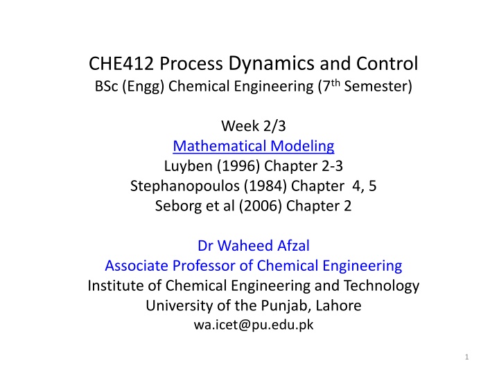
CHE412 Process Dynamics and Control BSc (Engg) Chemical Engineering (7thSemester) Week 2/3 Mathematical Modeling Luyben (1996) Chapter 2-3 Stephanopoulos (1984) Chapter 4, 5 Seborg et al (2006) Chapter 2 Dr Waheed Afzal Associate Professor of Chemical Engineering Institute of Chemical Engineering and Technology University of the Punjab, Lahore wa.icet@pu.edu.pk 1

Test yourself (and Define): Dynamics (of openloop and closedloop) systems Manipulated Variables Controlled/ Uncontrolled Variables Load/Disturbances Feedback, Feedforward and Inferential controls Error Offset (steady-state value of error) Set-point Stability Block diagram Transducer Final control element Mathematical model Input-out model, transfer function Deterministic and stochastic models Optimization Types of Feedback Controllers (P, PI, PID) Hint: Consult recommended books (and google!) Luyben (1996), Coughanower and LeBlanc (2008) 2

Types of Feedback Controllers Proportional: Proportional-Integral: c(t) = Kc (t) + cs ? ? ?? + ?? ? ? = ?? ? +?? ? 0 Proportional-Integral-Derivative: ? ? = ?? ? +?? ? ? ?? + ?? ? ? ??+ ?? ? 0 Nomenclature actuating output ? ? , error ? , gain ??, time constant ? Consult your class notes on modelling of stirred tank heater (t) 3 (Stephanopoulos, 1984)

Mathematical Modeling Mathematical representation of a process (chemical or physical) intended to promote qualitative and quantitative understanding Set of equations Steady state, unsteady state (transient) behavior Experimental Setup Inputs Outputs Compare Set of Equations (process model) Outputs Model should be in good agreement with experiments 4

Systematic Approach for Modelling (Seborg et al 2004) 1. Determine objectives, end-use, required details and accuracy 2. Draw schematic diagram and label all variables, parameters 3. Develop basis and list all assumptions; simplicity Vs reality 4. If spatial variables are important (partial or ordinary DEs) 5. Write conservation equations, introduce auxiliary equations 6. Never forget dimensional analysis while developing equations 7. Perform degree of freedom analysis to ensure solution 8. Simplify model by re-arranging equations 9. Classify variables (disturbances, controlled and manipulated variables, etc.) 5

Need of a Mathematical Model To understand the transient behavior, how inputs influence outputs, effects of recycles, bottlenecks To train the operating personnel (what will happen if , emergency situations , no/smaller than required reflux in distillation column, pump is not providing feed, etc.) Selection of control pairs (controlled v. / manipulated v.) and control configurations (process-based models) To troubleshoot Optimizing process conditions (most profitable scenarios) 6

Classification of Process Models based on how they are developed Theoretical Models based on principal of conservation- mass, energy, momentum and auxiliary relationships, , enthalpy, cp, phase equilibria, Arrhenius equation, etc) Empirical model based on large quantity of experimental data) Semi-empirical model (combination of theoretical and empirical models) Any available combination of theoretical principles and empirical correlations 7

Advantages of Different Models Theoretical Models Physical insight into the process Applicable over a wide range of conditions Time consuming (actual models consist of large number of equations) Availability of model parameters e.g. reaction rate coefficient, over-all heart transfer coefficient, etc. Empirical model Easier to develop but needs experimental data Applicable to narrow range of conditions 8

State Variables and State Equations State variables describe natural state of a process Fundamental quantities (mass, energy, momentum) are readily measurable in a process are described by measurable variables (T, P, x, F, V) State equations are derived from conservation principle (relates state variables with other variables) (Rate of accumulation) = (rate of input) (rate of output) + (rate of generation) - (rate of consumption) 9

Modeling Examples Jacketed CSTR Basis Flow rates are volumetric Compositions are molar A B, exothermic, first order Assumptions Perfect mixing , cP are constant Perfect insulation Coolant is perfectly mixed No thermal resistance of jacket Fi, CAi, Ti F, CA, T Coolant 10

Modeling of a Jacketed CSTR (Contd.) Overall Mass Balance (Rate of accumulation) = (rate of input) (rate of output) Component Mass Balance (Rate of accumulation of A) = (rate of input of A) (rate of output of A) + (rate of generation of A) (rate of consumption of A) Fi, CAi, Ti Coolant Fco,Tco V CA T F, CA, T Coolant Fci,Tci Energy Balance (Rate of energy accumulation) = (rate of energy input) (rate of energy output) - (rate of energy removal by coolant) + (rate of energy added by the exothermic reaction) 11

Modeling of a Jacketed CSTR (Contd.) Overall Mass Balance Fi, CAi, Ti ?? ??= ?? ? Coolant Fco,Tco V CA T Component Mass Balance ??? ?? ? =?? ??? ?? ???0? ?/?? F, CA, T Coolant Fci,Tci Energy Balance ?? ?? =?? Input variables: CAi, Fi, Ti, Q, (F) Output variables: V, CA, T ? ?? ? ? ? ?? ?0 ? ?/?? ?? ?? ? (??? ? ?? + 12 ? ???)

Degrees of Freedom (Nf) Analysis Nf = Nv - NE Case (1): Nf = 0 i.e. Nv = NE (exactly specified system) We can solve the model without difficulty Case (2): f > 0 i.e. Nv > NE (under specified system), infinite number of solutions because Nf process variables can be fixed arbitrarily. either specify variables (by measuring disturbances) or add controller equation/s Case (3): Nf < 0 i.e. Nv < NE (over specified system) set of equations has no solution remove Nf equation/s We must achieve Nf = 0 in order to simulate (solve) the model13

Stirred Tank Heater: Modeling and Degree of Freedom Analysis Basis/ Assumptions Perfectly mixed, Perfectly insulated , cPare constant Overall Mass Balance ?? ??= ?? ? Energy Balance ?? ??=?? Degree of Freedom Analysis Independent Equations: 2 Variables: 6 (h, Fi, F, Ti, T, Q) Nf= 6-2 (= 4) Underspecified A Steam Fst ? ? ?? ? ? ?? 14

Stirred Tank Heater: Modeling and Degree of Freedom Analysis Nf = 4 Specify load variables (or disturbance) Measure Fi, Ti (Nf = 4 - 2 = 2) Include controller equations (not studied yet); specify CV-MV pairs: A CV MV Steam Fst h F T Q ?? ??= ?? ? ??=?? ? = ?? + ??? ??? ? = ??+ ??? ???? ? ?? ? ? ?? ? ? ?? Nf = 2 - 2 = 0 Can you draw these control loops? 15

Modeling an Ideal Binary Distillation Column Basis/ Assumptions 1. Saturated feed 2. Perfect insulation of column 3. Trays are ideal 4. Vapor hold-up is negligible 5. Molar heats of vaporization of A and B are similar 6. Perfect mixing on each tray 7. Relative volatility ( ) is constant 8. Liquid holdup follows Francis weir formulae 9. Condenser and Reboiler dynamics are neglected 10. Total 20 trays, feed at 10 2, 4, 5 V1 = V2 = V3= VN (not valid for high-pressure columns) Condenser = 20 Reflux Drum mD F D xD R xD Z VB mB Reboiler B xB (Stephanopoulos, 1984) 16

Modeling Distillation Column V20 Reflux Drum Overall ?(??) ?? Component ??? ?? Top Tray Overall ?(?20) = ?20 ? ? mD D xD R xD = (?20/??)(?20 ??) Reflux Drum V20 = ? + ?19 ?20 ?20 R ?? N = 20 Top Tray V19 Component L20 ??20 ??= Remember V1 = V2= . VN = VB 1 ? ?? ?20 + ??(?19 ?20) ?20 17

Modeling Distillation Column LN+1 vN Nth Stage (stages 19 to 11 and 9 to 2) Overall ?(??) ?? Component ?(????) ?? Feed Stage (10th) Overall ?(?10) ?? Component ?(?10?10) ?? mN = ??+1+ ?? 1 ?? ?? Nth Stage LN vN-1 = ??+1??+1+ ?? 1?? 1 ???? ???? . simplify! L11 v10 F Z = ?11+ ? + ?9 ?10 ?10 mN Feed Stage (10th) L10 v9 = ?11?11+ ?? + ?9?9 ?10?10 ?10?10 18 . simplify!

Modeling Distillation Column 1st Stage Overall ?(?1) ?? Component 1st Stage V1 L2 L1 VB = ?2+?? ?1 ?1 ?(?1?1) ?? = ?2?2+ ???? ?1?1 ?1?1 Column Base Overall ?(??) ?? Component ?(????) ?? simplify! VB L1 = ?1 ? ?? VB mB Column Base = ?1?1 ??? ???? B 19 . simplify!

Modeling Distillation Column Equilibrium relationships (to determine y) Mass balance (total and component) around 6 segments of a distillation column: reflux drum, top tray, Nth tray, feed tray, 1st tray and column base. Solution of ODE for total mass balance gives liquid holdups (mN) Solution of ODE for component mass balance gives liquid compositions (xN) V1 = V2= = VN = VB (vapor holdups) How to calculate y (vapor composition) and L (liquid flow rate) Recall ij is constant throughout the column Use ij = ki/kj , xi + xj =1, yi + yj = 1, and k = y/x to prove ?? ?? ?+( ?? ?)??Phase-equilibrium relationship (recall thermodynamics) ??= 20

Modeling Distillation Column Hydraulic relationships (to determine L) Liquid flow rate can be calculated using well-known Francis weir hydraulic relationship; simple form of this equation is linearized version: ??= ??0+?? ??0 LN is flow rate of liquid coming from Nth stage LN0 is reference value of flow rate LN mN is liquid holdup at Nth stage mN0 is reference value of liquid holdup mN is hydraulic time constant (typically 3 to 6 seconds) 21

Modeling Distillation Column Degree of Freedom Analysis Total number of independent equations: Equilibrium relationships (y1, y2, yN, yB) Hydraulic relationships (L1, L2, LN) (does not work for liquid flow rates D and B) Total mass balances (1 for each tray, reflux drum and column base) Total component mass balances (1 for each tray, reflux drum and column base) Total Number of equations NE = 4N + 5 (85) 44 differential and 41 algebraic equations Note the size of modeleven for a simple system with several simplifying assumptions! N+1 (21) N (20) N+2 (22) N+2 (22) 22

Modeling Distillation Column Degree of Freedom Analysis Total number of independent variables: Liquid composition (x1, x2, xN, xD,xB) N+2 Liquid holdup (m1, m2, mN, mD,mB) N+2 Vapor composition (y1, y2, yN, yB) Liquid flow rates (L1, L2, LN) Additional variables (Feed: F, Z; Reflux: D, R; Bottom: B, VB) Total Number of independent variables NV = 4N + 11 N+1 N 6 Degree of Freedom = (4N + 11) (4N + 5) System is underspecified = 6 23

Modeling Distillation Column Degree of Freedom Analysis (4N + 11) (4N + 5) = 6 Specify disturbances: F, Z Include controller equations (Recall our discussion on types of feedback controllers ) General form, of P-Controller (Nf = 6-2 = 4) c(t) = cs + Kc (t) Controller Equation (Proportional Controller) Controlled Variable Manipulated Variable xD R R = Kc (xs - xD) + Rs VB = Kc (xBs-xB) + VBs D = Kc (mDs-mD) + Ds B = Kc (mBs-mB) + Bs xB VB mD D mB B Nf = 4 - 4 = 0 Can you draw these four feedback control loops? 24

CV MV loop Feedback Control on a Binary Distillation Column xD xB mD mB R 1 VB D 2 3 B 4 R (Stephanopoulos, 1984) 25

Week 2/3 Weekly Take-Home Assignment 1. 2. Define all the terms on slide 2 with examples whenever possible. Prepare short answers to things to think about (Stephanopoulos, 1984) page 33-35 Prepare short answers to things to think about (Stephanopoulos, 1984) page 78-79 Solve the following problems (Chapter 4 and 5 of Stephanopoulos, 1984): II.1 to II.14, II.22, II.23 (Compulsory) 3. 4. Submit before Friday Curriculum and handouts are posted at: http://faculty.waheed-afzal1.pu.edu.pk/ 26