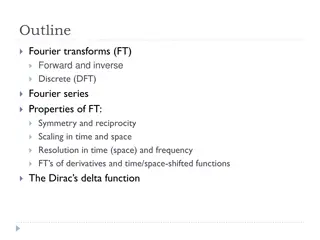
Properties of Continuous-Time Fourier Transform and Functions
Discover the properties and transformations of the continuous-time Fourier transform, including linearity, time scaling, time reversal, time shifting, frequency shifting, symmetry properties, and Fourier transform for real functions. Explore the Fourier transform for real and even/odd functions, understanding their characteristics and spectral representations.

Download Presentation

Please find below an Image/Link to download the presentation.
The content on the website is provided AS IS for your information and personal use only. It may not be sold, licensed, or shared on other websites without obtaining consent from the author. If you encounter any issues during the download, it is possible that the publisher has removed the file from their server.
You are allowed to download the files provided on this website for personal or commercial use, subject to the condition that they are used lawfully. All files are the property of their respective owners.
The content on the website is provided AS IS for your information and personal use only. It may not be sold, licensed, or shared on other websites without obtaining consent from the author.
E N D
Presentation Transcript
Continuous-Time Fourier Transform Properties of Fourier Transform
Notation = [ ( )] ( ) f t F j F = 1 - [ ( )] ( ) F j f t F ( ) ( ) F f t F j
Linearity + + ( ) ( ) ( ) ( ) F a f t a f t a F j a F j 1 1 2 2 1 1 2 2
Time Scaling j 1 ( ) F f at F | | a a
Time Reversal ( ) ( ) F f t F j Pf) = t = = j t j t [ ( )] ( ) ( ) f t f t e dt f t e dt F = = = t = t = t = j t ( ) ( ) f t e d t j t ( ) ( ) f t e d t = t = t = = t t = = j t j t ( ) ( ) f t e dt f t e dt = t t = = ( ) F j j t ( ) f t e dt
Time Shifting ( ) j t ( ) F f t t F j e 0 0 Pf) = t = = j t j t [ ( )] ( ) ( ) f t t f t t e dt f t t e dt F 0 0 0 = t + = t t = + + ( ) j t t 0 ( ) ( ) f t e d t t 0 0 + = t t 0 = t j = t j t ( ) e f t e dt 0 = t j = j t = t ( ) j t F j e ( ) e f t e dt 0 0
Frequency Shifting (Modulation) ) 0 j ( ) ( F f t e F j 0 Pf) = j t j t j t [ ( ) ] ( ) f t e f t e e dt F 0 0 = ( ) j t ( ) f t e dt 0 ) 0 = ( F j
Symmetry Property = [ ( )] 2 ( ) F jt f F Pf) d = j t 2 ( ) ( ) f t F j e = j t 2 ( ) ( ) f t F j e d Interchange symbols and t = [ ( )] F jt = j t F 2 ( ) ( ) f F jt e dt
Fourier Transform for Real Functions If f(t) is a real function, and F(j ) = FR(j ) + jFI(j ) F( j ) = F*(j ) = j t ( ) ( ) F j f t e dt = = j t * ( ) ( ) ( ) F j f t e dt F j
Fourier Transform for Fourier Transform for Real Functions Real Functions If f(t) is a real function, and F(j ) = FR(j ) + jFI(j ) F( j ) = F*(j ) FR(j ) is even, and FI(j ) is odd. FR( j ) = FR(j ) FI( j ) = FI(j ) Magnitude spectrum |F(j )| is even, and phase spectrum ( )is odd.
Fourier Transform for Fourier Transform for Real Functions Real Functions If f(t) is real and evenF(j ) is real If f(t) is real and odd F(j ) is pure imaginary Pf) Pf) = F = ) = Even Odd ( ( ) j ( ) ( ( ) j ( F ) f t f = t ( f t f t ( ) ) ) F j F j j = j = Real Real ( ) * ( ) ( ) * ( ) F j F j F F = = ( ) * ( ) ( ) * ( ) F j F j F j F j
Example: t = = [ ( ) cos ] ? f t [ ( )] ( ) f t F j F F 0 Sol) 1 + = j t j t ( ) cos ( )( ) f t t f t e e 0 0 0 2 1 1 = + j t j t [ ( ) cos ] [ ( ) ] [ ( ) ] f t t f t e f t e F F F 0 0 0 2 1 2 1 = + + [ ( )] [ ( )] F j F j 0 0 2 2
Example: f(t)=wd(t)cos 0t wd(t) 1 t t d/2 d/2 d/2 d/2 2 d / 2 d = = = j t ( ) [ ( )] sin W j w t e dt F d d 2 / 2 d d d + sin ( ) sin ( ) 0 0 2 2 = + = ( ) [ ( ) cos ] F j w t 0t F + d 0 0
1.5 d=2 0=5 1 Example: F(j ) 0.5 0 -0.5 -60 -40 -20 0 20 40 60 f(t)=wd(t)cos 0t wd(t) 1 t t d/2 d/2 d/2 d/2 2 d / 2 d j j = = = t ( ) [ ( )] sin W w t e dt F d d 2 / 2 d d d + sin ( ) sin ( ) 0 0 2 2 = + = ( ) [ ( ) cos ] F j w t 0t F + d 0 0
wd(t) 1 Example: t d/2 d/2 =sin at = ( ) f t ( ) ? F j t Sol) 2 d = ( ) sin Wd j 2 2 t sin td = = [ ( )] sin 2 ( ) W jt w F F d d 2 0 | | a at = = = [ ( )] ( ) f t w F F 2 a t 1 | | a
Fourier Transform of f(t) ( ) = ( ) and lim t ( ) 0 F f t F j f t ( ' ) ( ) F f t j F j Pf) = j t [ ( ' )] ( ' ) f t f t e dt F = + j t j t ( ) ( ) f t e j f t e dt = ( j ) j F
Fourier Transform of f (n)(t) ( ) j = ( ) and lim t ( ) 0 F f t F f t ( ) n n ( ) ( ) ( ) F f t j F j
Fourier Transform of f (n)(t) ( ) j = ( ) and lim t ( ) 0 F f t F f t j j ( ) n n ( ) ( ) ( ) F f t F
Fourier Transform of Integral ( ) ( ) 0 = = ( ) and ( ) 0 F f t F j f t dt F 1 ( ) t = ( dx ) f x F j F j t F = = ( ) ( dx ) t f x lim t j ( ) 0 t Let ( ' = = = [ )] [ 1 j ( )] ( ) ( ) t f t F j j F = ( ) ( ) j F j
The Derivative of Fourier Transform ( ) dF j [ ( )] F jtf t F d Pf) = j t ( ) ( ) F j f t e dt d ( ) dF j = = j t j t ( ) ( ) f t e dt f t e dt d d =F = [ ( )] jtf t j t [ ( )] jtf t e dt
Continuous-Time Fourier Transform Convolution
Basic Concept fo(t)=L[fi(t)] fi(t) Linear System fi(t)=a1fi1(t) + a2fi2(t) fo(t)=L[a1fi1(t) + a2fi2(t)] fo(t) = a1L[fi1(t)] + a2L[fi2(t)] = a1fo1(t) + a2fo2(t) A linear system satisfies
Basic Concept fo(t) fi(t) Time Invariant System fi(t +t0) fi(t t0) fo(t + t0) fo(t t0) fi(t) fo(t) t t fi(t+t0) fo(t+t0) t t fi(t t0) fo(t t0) t t
Basic Concept fo(t) fi(t) Causal System A causal system satisfies fi(t) = 0 for t < t0 fo(t) = 0 for t < t0
Which of the following systems are causal? Basic Concept fo(t) fi(t) Causal System fi(t) fo(t) t t t0 t0 fi(t) fo(t) t t t0 t0 fi(t) fo(t) t t t0 t0
Unit Impulse Response h(t)=L[ (t)] (t) LTI System f(t) L[f(t)]=? Facts: = = ( ) ( ) ( ) ( ) ( ) f t d f t d f t = = ( ) [ ( )] f L t d [ ( )] ( ) ( ) L f t L f t d Convolution = ( ) ( ) f h t d
Unit Impulse Response h(t)=L[ (t)] (t) LTI System f(t) [ L L[f(t)]=? * ) ( Facts: ( = f )] = h = f ( f ( )] ) f f t t ) t ( ) ( ) ( ) ( ) ( t d t d t = = ( ) [ ( f L t d [ ( )] ) ( ) L f t L f t d Convolution = ( ) ( ) f h t d
Unit Impulse Response Impulse Response LTI System h(t) f(t) f(t)*h(t)
Convolution Definition The convolution of two functions f1(t) and f2(t) is defined as: = ( ) ( ) ( ) f t f f t d 1 2 = ( ) * ( ) f t f t 1 2
Properties of Convolution = ( ) * ( ) ( ) * ( ) f t f t f t f t 1 2 2 1 = = = ( ) * ( ) ( ) ( ) ( ) ( ) f t f t f f t d f f t d 1 2 1 2 1 2 = = t = ] ) ( ) [ ( ( ) f t f t t d t 1 2 = t = = = ( ) ( ) f t f d 1 2 = f = ( ) * ( ) f t f t ( ) ( ) t f d 2 1 1 2
Properties of Convolution = ( ) * ( ) ( ) * ( ) f t f t f t f t 1 2 2 1 f(t) f(t)*h(t) Impulse Response LTI System h(t) h(t)*f(t) h(t) Impulse Response LTI System f(t)
Properties of Convolution = [ ( ) * ( )] * ( ) ( [ * ) ( ) * ( )] f t f t f t f t f t f t 1 2 3 1 2 3
The following two systems are identical Properties of Convolution = [ ( ) * ( )] * ( ) ( [ * ) ( ) * ( )] f t f t f t f t f t f t 1 2 3 1 2 3 h1(t) h2(t) h3(t) h2(t) h3(t) h1(t)
Properties of Convolution = ( ) * ( ) ( ) f t t f t f(t) f(t) (t) = ( ) * ( ) ( ) ( ) f t t f t d = = ( ) ( ) f t d (t ) f
Properties of Convolution = ( ) * ( ) ( ) f t t f t f(t) f(t) (t) = ( ) * ( ) ( ) f t t T f t T = ( ) * ( ) ( ) ( ) f t t T f t T d = = ( ) ( ) f t T d ( ) f t T
Properties of Convolution = ( ) * ( ) ( ) f t t T f t T (t T) f(t) f(t T) 0 T f(t) f(t) t t 0 0 T
System function (tT) serves as an ideal delay or a copier. Properties of Convolution = ( ) * ( ) ( ) f t t T f t T (t T) f(t) f(t T) 0 T f(t) f(t) t t 0 0 T
Properties of Convolution ( ) * ( ) ( ) ( ) F f t f t F j F j 1 2 1 2 j = t [ ( ) * ( )] ( ) ( ) F f t f t f f t d e dt 1 2 1 2 = j t ( ) ( ) f f t e dt d 1 2 = j ( ) ( ) f F j e d 1 2 = = j ( ) ( ) F j F j ( ) ( ) F j f e d 1 2 2 1
Time Domain Frequency Domain convolution multiplication Properties of Convolution ( ) * ( ) ( ) ( ) F f t f t F j F j 1 2 1 2 j = t [ ( ) * ( )] ( ) ( ) F f t f t f f t d e dt 1 2 1 2 = j t ( ) ( ) f f t e dt d 1 2 = j ( ) ( ) f F j e d 1 2 = j j = j ( ) ( ) ( ) ( ) F F F j f e d 2 1 1 2
Time Domain Frequency Domain convolution multiplication Properties of Convolution j j ( ) * ( ) ( ) ( ) F f t f t F F 1 2 1 2 Impulse Response LTI System h(t) f(t) f(t)*h(t) Impulse Response LTI System H(j ) F(j ) F(j )H(j )
Time Domain Frequency Domain convolution multiplication Properties of Convolution j j ( ) * ( ) ( ) ( ) F f t f t F F 1 2 1 2 F(j )H1(j )H2(j )H3(j ) F(j )H1(j ) H1(j ) H2(j ) H3(j ) F(j ) F(j )H1(j )H2(j )
Properties of Convolution j j ( ) * ( ) ( ) ( ) F f t f t F F 1 2 1 2 Fo(j ) H(j ) Fi(j ) 1 p p 0 0 0 An Ideal Low-Pass Filter
Properties of Convolution j j ( ) * ( ) ( ) ( ) F f t f t F F 1 2 1 2 Fo(j ) H(j ) Fi(j ) 1 p p 0 0 0 An Ideal High-Pass Filter
Properties of Convolution 1 ( ) ( ) ( ) [ ( )] F f t f t F j F j d 1 2 1 2 2 1 ( ) ( ) ( ) * ( ) F f t f t F j F j 1 2 1 2 2
Time Domain Frequency Domain multiplication convolution Properties of Convolution 1 ( ) ( ) ( ) [ ( )] F f t f t F j F j d 1 2 1 2 2 1 j j ( ) ( ) ( ) * ( ) F f t f t F F 1 2 1 2 2


")


")
")
(t)")
(t)")


 serves as")