Properties of the Laplace Transform in Pattern Recognition and Signal Processing

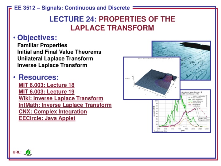
ECE 8443 Pattern Recognition EE 3512 Signals: Continuous and Discrete LECTURE 24: PROPERTIES OF THE LAPLACE TRANSFORM Objectives: Familiar Properties Initial and Final Value Theorems Unilateral Laplace Transform Inverse Laplace Transform Resources: MIT 6.003: Lecture 18 MIT 6.003: Lecture 19 Wiki: Inverse Laplace Transform IntMath: Inverse Laplace Transform CNX: Complex Integration EECircle: Java Applet URL:

Familiar Properties of Linear Transforms To introduce the inverse Laplace transform and some important applications of the transform (e.g., circuits), we will need to introduce some familiar properties of the transform (e.g., linearity). There are some properties unique to the Laplace transform (e.g., the Initial Value Theorem). There are some properties of the Fourier Transform that do not have an equivalent for the Laplace transform (e.g., duality, Parseval s theorem). Linearity: ax + + ( ) ( ) ( ) ( ) t bx t aX s bX s 1 2 1 2 Note that the ROC for the sum is at least the intersection of the ROCs for each component (it must include regions for which both transforms converge, as we demonstrated in lecture 21). In some special cases, the ROC can be larger (e.g., when the zeroes of one component cancel the poles of the other component). For example: 0 ) ( ) ( ) ( and 2 1 t x t x t x b a = = = ROC is the entire - plane s Example: ) ( t x ) 1 + s + 1 s 1 + ( 2 1 s s s = + = + = + = t ( ) ( ) ( ) u t e u t X s ) 1 + ) 1 + ) 1 + 1 ( )( ( )( ( )( s s s s s s EE 3512: Lecture 24, Slide 1

Properties of the Laplace Transform Time-Shift: sT ( ) ( ) same ROC as x t T e X s X(s) Example: 1 + = 2 t ( ) ( ) ROC : Re{ } 2 e u t X s X(s) 2 s 3 s e ( 2 ) 3 = t ( ) 3 ( ) ROC : Re{ } 2 e u t X s X(s) + 2 s Note that the ROC doesn t change because it is defined by the pole location. Example: Ts Ts 1 1 e e = = = ( ) ( ) ( ) ( ) x t u t u t T X s s s s What is the ROC? Hint: This is a time-limited signal. Time Scaling: 1 a s ( ) ( ) x at X a Example: 1 1 1 = ( ) ( ) u at Is this result expected? s a s a / EE 3512: Lecture 24, Slide 2

More Properties Multiplication by a Power of t: n d ) 1 n n ( ) ( ( ) same ROC as t x t X s X(s) n ds Compare to Fourier transform: d j t x t n j n n ( ) ( ) ( ) X e n ds Example: ) ( t r 1 1 s 1 s d = = ) 1 = 1 ( ) ( ) ( ( ) tu t R s 1 2 ds Time-Domain Differentiation (Bilateral): ) ( s X s dt n d x t n ( ) ROC can be bigger than the ROC for ( ) x t n Example: ( ) 1 s du t = = = = ( ) ( ) ( ) ( )( ) 1 ROC for ( ) is larger than the ROC for ( ) x t t X s s t u t dt Integration: t 1 s = ( ) ( ) ROC must not include 0 x d X s s 0 EE 3512: Lecture 24, Slide 3

Convolution The convolution integral: (t ) x ( ) * ( ) x t h t CT LTI (t h t = = ( ( ) ( ) * ( ) ) ( ) y t x t h t x h t d ) Laplace transform is analogous to the Fourier transform: ) ( ) ( ) ( s H s X s Y = But, because the Laplace transform and its inverse (to be discussed in a moment) are not symmetric, the dual of this is not true: ) ( * ) ( ) ( ) ( s H s X t h t x This is one reason the Fourier transform is more popular for applications involving communications systems and modulation. The ROC is at least the overlap of the ROCs for each signal (again, it can be larger than the ROC for either signal). Example: 1 ) ( ) 1 ( ) ( ) ( s s e = = x t u t u t X s 2 + 2 s s s 1 1 2 e e e s = = = 2 ( ) ( ) * ( ) ( ) y t x t x t X s 2 s s 2 s 1 s e e = + = ) 1 ) 1 + 1 1 1 L L L ( ) { } 2 { } { } ( ) ( 2 ( ( ) 2 ( ) 2 y s tu t t u t t u t 2 2 2 s s EE 3512: Lecture 24, Slide 4

The Unilateral (One-sided) Laplace Transform Define a special case of the Laplace transform for right-sided signals: 0 = st ( ) ( ) X s x t e dt = For right-sided signals ( ), and for causal systems ( ), the one-sided and two-sided transforms are equal. = ( ) , 0 0 ( ) , 0 0 h t t x t t Several properties change slightly, such as differentiation: ) ( x s sX dt dt 2 ( ) dx t d x t dx ) 2 ( ) 0 ( ) ( ) 0 ( s X s sx 2 dt = 0 t Proof: ( ) ( ) ( ) dx t dx t dx t = = + st st st UL ( ) (using integratio n by parts) e dt x t e s e dt dt dt dt 0 0 0 = + 0 ( x ) ( ) sX s Other properties, such as convolution, hold as is, as long as the system is causal and the input starts at t = 0. EE 3512: Lecture 24, Slide 5

Initial and Final Value Theorems = Theorem: ) 0 ( x lim s ( ) (Initial Value Theorem) sX s = x( ) lim s ( ) (Final Value Theorem) sX s Proof: 0 Applying the differentiation property: ) ( s sX dt dx t = UL ( ) ) 0 ( x ( ) dx t = ) 0 ( 0 dt s dt ( ) ( ) dx t dx t = = st UL e dt 0 ( ) dt dt dx t = ) 1 ( ( ) ) 0 ( x 0 dt x s 0 dt 0 Combining s sX the = two : = ( ) ) 0 ( x 0 ) 0 ( x lim s ( ) s sX s = = ( ) ) 0 ( x ( ) ) 0 ( x 0 ( ) lim s ( ) x sX s s x sX s 0 The initial value theorem can be extended to higher-order derivatives: ) ( 2 sx s X s dt t = dx t = lim s [ ( ) 0 ( )] 0 Allow initial and final conditions to be computed directly from the transform. EE 3512: Lecture 24, Slide 6

Application of the Initial and Final Value Theorems Consider a rational transform: ) ( ) ( s D : order of N(s) n N s = where X s : order of D(s) d ( ) Initial value: + 0 1 d n + 1 n s = = = = + ) 0 ( x lim s ( ) lim s 0 1 sX s finite d n d s + 1 d n For example: 1 1 + s = = = ( ) ) 0 ( x lim s 1 X s 1 1 s s 1 1 s = = = ( ) ) 0 ( x lim s 0 X s ) 1 + 2 2 ( s s Final Value: = = 0 = x( ) lim s ( ) 0 lim s ( ) poles no at s sX s X s 0 0 1 + s = = = ( ) ( ) lim s 1 X s x + 1 1 s s s 0 1 = = = ( ) ( ) lim s 0 X s x ) 1 + ) 1 + 2 2 ( ( s s 0 EE 3512: Lecture 24, Slide 7

Inverse Laplace Transform using Complex Integration = = + Recall: st ( ) ( ) , ROC X s x t e dt s j F = t ( ) x t e Choose ROC and apply the inverse Fourier transform: 1 ( ) j = + j d t t ( ) x t e X e 2 1 ( ) ( + j = + j d ) t ( ) x t X e 2 But for a fixed , s = + j , ds = j d : + j X 1 1 ( ) s C = = st st ( ) ( ) x t e ds X s e ds 2 2 j j j This is a contour integral in the complex plane. Such integrals are studied extensively in a course on complex variables, but are beyond the scope of this course. EE 3512: Lecture 24, Slide 8

Specific Cases of Inverse Laplace Transforms We will restrict ourselves to two special case: 1) Rational transforms: use partial fractions expansion ) ( ) ( + + b s a s s D N s A B = = + + ... X s ( ) 2) Exponentials: use the shift property: = + + = + + sT sT ( ) ( ) ( ) ... ( ) ( ) ( ) ... X s e X s e X s x t x t T x t T 1 2 1 2 1 1 2 2 These two building blocks will allow us to construct the inverse transforms for many common signals and systems, including those used in circuit analysis. Therefore, the unilateral Laplace transform can be applied to finding both the transient and steady-state responses (as well as the frequency response) of a circuit. This is one of its principal uses in electrical engineering. The use of partial fractions, however, requires being able to factor a polynomial into its roots. You have previously used this in calculus, and have good MATLAB support for this as well. EE 3512: Lecture 24, Slide 9

Summary Review your tables of transform properties (one-sided!) and common transform pairs: x.jpg EE 3512: Lecture 24, Slide 10