Properties of Z-Transform and Inverse Z-Transform Lecture Overview

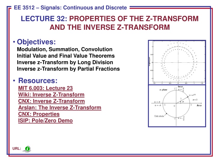
ECE 8443 Pattern Recognition EE 3512 Signals: Continuous and Discrete LECTURE 32: PROPERTIES OF THE Z-TRANSFORM AND THE INVERSE Z-TRANSFORM Objectives: Modulation, Summation, Convolution Initial Value and Final Value Theorems Inverse z-Transform by Long Division Inverse z-Transform by Partial Fractions Resources: MIT 6.003: Lecture 23 Wiki: Inverse Z-Transform CNX: Inverse Z-Transform Arslan: The Inverse Z-Transform CNX: Properties ISIP: Pole/Zero Demo URL:

Properties of the z-Transform + + Linearity: [ ] [ ] [ ] [ ] ax n bx n aX z bX z 1 2 1 2 n [ ] [ ] x n n z X dX z [ Time-shift: 0 0 ] z Multiplication by n: [ ] nx n z dz = = n Proof: [ ] X(z) x n z n ( ) ( ) dX z dX z ] n = = = = = 1 n n Z [ ] [ ] [ n x n z z n x n z nx dz dz n n z Multiplication by an: an [ ] x n X a n z z = n = n Proof: = = = n n n Z ( e ( ) ( [ ]) [ ] a u n a x n z x n X a a ) z ( e ( X X Multiplication by ej n: j n j n [ ] e x n X ) ) ( ) Multiplication by cos n: + ) j n j n cos( ) [ ] / 1 ( ) 2 n x n z X e ( z Multiplication by sin n: j n j n sin( ) [ ] ( ) 2 / n x n j e z X e z 1 n = Summation: = [ ] [ ] ( ) ( ) v n x i V z X z 1 1 z = 0 i EE 3512: Lecture 32, Slide 1

Convolution = Convolution: [ ] * [ ] [ ] [ ] ( ) ( ) x n h n x k h n k X z H z = k k n Proof: = = n Z Z [ ] * [ ] [ ] [ ] [ ] [ ] x n h n x k h n k x k h n k z = = = k k n = n [ ] [ ] x k h n k z = = = Change of index on the second sum: m n k + = = ( ) ) m i k m Z [ ] * [ ] [ ] [ ] [ ] [ ] x n h n x k h m z x k z h m z = = = = k m k m = ( ) ( ) X z H z The ROC is at least the intersection of the ROCs of x[n] and h[n], but can be a larger region if there is pole/zero cancellation. The system transfer function is completely analogous to the CT case: = n 0 0 ] [ = n n h = n [ ] ( ) [ ] h n H z h n z Causality: Implies the ROC must be the exterior of a circle and include z = . EE 3512: Lecture 32, Slide 2

Initial-Value and Final-Value Theorems (One-Sided ZT) Initial Value Theorem: = ] 0 [ x lim z = ( ) X z = + + = Proof: 1 n lim z ( ) lim z [ ] lim z ] 0 [ x ] 1 [ x ... ] 0 [ x X z x n z z = 0 n = ) 1 lim n [ ] lim z ( ( ) x n z X z Final Value Theorem: 1 + z + z 2 2 3 2 4 3 2 4 z z z z = = Example: ( ) X z 5 . 1 + 5 . 0 ) 5 . 0 + 3 2 2 2 ( 1 )( z z z z + 2 3 z 2 4 5 z z = ) 1 = = = lim n [ ] [( ( )] 10 x n z X z 5 . 0 + = 2 1 5 . z z = 1 z Tables 7.2 and 7.3 in the textbook contain a summary of the z-Transform properties and common transform pairs. EE 3512: Lecture 32, Slide 3

Inverse Laplace Transform Recall the definition of the inverse Laplace transform via contour integration: + st st ds e s X j j 2 2 j 1 1 ( ) s C = = ( ) ( ) x t X e ds j The inverse z-transform follows from this: C j 2 1 = 1 ndz [ ] ( ) x n X z z Evaluation of this integral is beyond the scope of this course. Instead, as with the Laplace transform, we will restrict our interest in the inverse transform to rational forms (ratio of polynomials). We will see shortly that this is convenient since linear constant-coefficient difference equations can be converted to polynomials using the z-transform. As with the Laplace transform, there are two common approaches: Long Division Partial Fractions Expansion Expansion by long division Is also known as the power series expansion approach and can be easily demonstrated by an example. EE 3512: Lecture 32, Slide 4

Long Division z 2 1 + z Consider: = ( ) X z + 3 2 4 z Solution: + 1 2 3 4 0 3 4 z z z z + + 3 2 1 2 4 1 z z z z + + 3 2 2 4 1 z z z + + 2 1 2 4 z z + + 2 1 2 4 z z 1 3 4 z 1 3 4 z 2 3 3 6 12 z z + + 1 2 3 4 6 12 z z z + 1 2 3 0 3 z z z + + 3 2 2 4 1 1 3 4 z z z 4 8 16 z z z + + 2 1 2 4 z z + + 2 3 4 6 20 16 z z z 1 3 4 z 2 3 3 6 12 z z + + 1 2 3 4 6 12 z z z = + n + 1 2 3 4 ( n ) 0 + 3 4 ... X z z z z z Implications of stability? = ] 1 + [ ] 0 [ ] 1 [ 3 [ ] 3 4 [ ] 4 ... x n n n EE 3512: Lecture 32, Slide 5

Inverse z-Transform Using MATLAB + 3 2 8 z 2 5 z z z Consider: = ( ) X z . 1 + 3 75 75 . z MATLAB: Syms X x z X = (8*z^3+2*z^2-5*z)/(z^3-1.75*z+.75); x = iztrans(X) x = 2*(1/2)^n+2*(-3/2)^n+4 Evaluate numerically: num = [8 2 -5 0]; den = [1 0 -1.75 .75]; x = filter(num, den, [1 zeros(1,9)]) Output: 8 2 9 -2.5 14.25 -11.125 26.8125 -30.1563 55.2656 EE 3512: Lecture 32, Slide 6

Inverse z-Transform Using Partial Fractions Rational transforms can be factored using the same partial fractions approach we used for the Laplace transforms. The partial fractions approach is preferred if we want a closed-form solution rather than the numerical solution long division provides. 1 ) ( 2 3 z z z + 3 z = X z Example: 2 In this example, the order of the numerator and denominator are the same. For this case, we can use a trick of factoring X(z)/z: = = 5 . 0 + + c 5 . 0 + c 3 2 ( ) 2 ( 2 )( . 0 j 866 )( . 0 j 866 ) A z z z z z z z c c ( z ) X z = + + + 0 3 1 1 + + 5 . 0 + 5 . 0 z . 0 j 866 . 0 j 866 2 z z z z ( z ) 1 X z = = = 5 . 0 ( ) c 0 2 = 0 z ( z ) X z ( ) = 5 . 0 + + = + . 0 j 866 . 0 429 0825 . 0 j c z 1 = 5 . 0 . 0 j 866 z ( z ) X z ( ) = = 2 . 0 643 c z 3 = 2 z EE 3512: Lecture 32, Slide 7

Inverse z-Transform (Cont.) We can compute the inverse using our table of common transforms: c j z + + + c z c z z = + + + 3 1 1 ( ) X z c 0 5 . 0 . 0 866 5 . 0 . 0 c 866 2 z j z c c = + + + 3 1 1 c 0 + + + 1 1 1 1 n 5 . 0 c + . 0 j 866 1 5 . 0 n . 0 j 866 1 2 z z + z = 5 . 0 + 5 . 0 + n n n [ ] [ ] ( . 0 j 866 ) [ ] ( . 0 j 866 ) [ ] 2 [ ] x n c u c u n c u n 0 1 1 3 The exponential terms can be converted to a single cosine using a magnitude/phase conversion: = . 0 ( + = 2 2 ) 5 . 0 ( 866 ) 1 p 1 . 0 866 4 = + = 1 tan rad p 1 5 . 0 3 = . 0 ( + = 2 2 . 0 ( 429 ) 0825 ) . 0 437 c 1 0825 . 0 = = 1 tan . 0 19 rad (10.89 ) c 1 . 0 + 429 c + = 5 . 0 + 5 . 0 + + n n n [ ] [ ] ( . 0 j 866 ) [ ] ( . 0 j 866 ) [ ] 2 [ ] x n c n u n c u n c u n 0 1 1 c 3 = + + n [ ] 2 cos( ) ) 2 ( 3 [ ] c n c p p n c u n 0 1 1 1 1 4 = 5 . 0 + + + n [ ] . 0 874 cos( . 0 19 ) . 0 643 ) 2 ( [ ] n n u n 3 EE 3512: Lecture 32, Slide 8

Inverse z-Transform (Cont.) This can be verified using MATLAB: num = [1 0 0 1]; den = [1 -1 -1 -2 0]; [r, p] = residue(num, den) r = 0.6429 0.4286 0.825i 0.4286 + 0.825i -0.5000 + 3 1 z = ( ) X z 3 2 2 z z z p= 2.0000 -0.5000 + 0.8660i -0.5000 0.8660i 0 The first 20 samples of the output can be computed numerically using: num = [1 0 0 1]; den = [1 -1 -1 -2 0]; x = filter(num, den, [1 zeros(1,19)]); Using MATLAB as a resource for solving homework problems can greatly reduce the time you spend doing busywork. EE 3512: Lecture 32, Slide 9

Summary Introduced additional properties of the z-transform. Derived the convolution property for DT LTI systems. Introduced two practical ways to compute the inverse z-transform: long division and partial fractions expansion. Worked examples of each and demonstrated how to solve these problems using MATLAB. EE 3512: Lecture 32, Slide 10