Pulse Propagation on Transmission Lines: Visualizing Wave Travel
This set of notes delves into the concept of pulse propagation on transmission lines, highlighting the visualization of wave travel, pulse shapes, voltage signals, and oscilloscope displays. The discussion covers understanding wave behaviors, wave reflections, forward waves, voltage pulse delays, and mirror-image effects. By examining voltage wave snapshots at fixed times and positions, the notes elucidate the relationship between time and space in wave propagation scenarios.

Download Presentation

Please find below an Image/Link to download the presentation.
The content on the website is provided AS IS for your information and personal use only. It may not be sold, licensed, or shared on other websites without obtaining consent from the author.If you encounter any issues during the download, it is possible that the publisher has removed the file from their server.
You are allowed to download the files provided on this website for personal or commercial use, subject to the condition that they are used lawfully. All files are the property of their respective owners.
The content on the website is provided AS IS for your information and personal use only. It may not be sold, licensed, or shared on other websites without obtaining consent from the author.
E N D
Presentation Transcript
ECE 3317 Applied Electromagnetic Waves Prof. David R. Jackson Fall 2024 Notes 7 Transmission Lines (Pulse Propagation and Reflection) 1
Pulse on Transmission Line (cont.) ( ) , i z t + - ( ) , v z t z Convenient for visualizing a wave traveling on the line (a snapshot ). ( ) ( ) ( ) = + + , v z t F z c t G z c t d d ( ) ( ) + Alternative notation: , v z t , v z t ( ) ( ) ( ) = + + , / / v z t f t z c g t z c d d Convenient for seeing what an oscilloscope on the line will display. (In this set of notes we will be using the second form.) 2
Pulse on Transmission Line A voltage signal is applied at the input of a semi-infinite transmission line. ( ) + = , i i z t z + + ( ) ( ) t + = Z , v v z t gv 0 - ( ( ) ) + , , v i z t z t z = 0 = Z 0 + Sawtooth wave voltage pulse Example: 0 V ( ) t gv t t 3
Pulse on Transmission Line (cont.) + + ( ) t ( ) + = Z gv , v v z t 0 - z = 0 We have only a forward wave. ( ) ( ) + = , / v z t f t z c d ( ) ( ) + = What is the function f ? 0, v t f t Set z = 0: ( ) ( ) t + = 0, v t v Also, we have: g ( ) ( ) t = f t v g Hence ( ) ( ) + = , / v z t v t z c g d 4
Pulse on Transmission Line (cont.) ( ) ( ) + = , / v z t v t z c g d At any position z, the voltage pulse (oscilloscope trace) that is measured is the same as the input voltage pulse from the generator, except that it is delayed by a time td =z / cd. z 0 z = 0 = / t z c ( ) + ( ) , v z t d d + , v z t t t t t 5
Pulse on Transmission Line (cont.) Note the delay in the trace on this oscilloscope. Time delay: = / t z c d d + Z ( ) t gv 0 z z = 0 0 Here is what oscilloscopes will show. ( ) ( ) + = , / v z t v t z c g d 6
Pulse on Transmission Line (cont.) = t t Snapshot of voltage wave at a fixed time. 0 Pulse = z c t 0 0 d + + ( ) ( ) t + Z , v z t gv = z c t 0 d - z = 0 Note that the shape of the pulse as a function of z is a scaled mirror image of the pulse shape as a function of t. ( ) 0 V gv ( ) ( ) + = , / v z t v t z c 0 0 g d / t z c 0 d Note the minus sign! This causes the mirror-image effect. t 7
Pulse on Transmission Line (cont.) This voltage waveform moves past the oscilloscope to create the trace. (The oscilloscope trace is the mirror image of the snapshot shape.) = / t z c Time delay: d d dc Pulse + + ( ) ( ) t Z + , v z t gv = z c t 0 d - z z = 0 0 8
Pulse on Transmission Line (cont.) The pulse is shown emerging from the source end of the line. A series of snapshots is shown. dc = t t t 1 = = = = t t t t t t t t t 2 3 2 4 3 t = 0 ( ) t = +- z c t gv = z c t 1 d d z = 0 ( ) ( ) + = , / v z t v t z c g d ( ) t gv t t 9
Step Function Source Another example (battery and switch) t = 0 + - ( ) t 1 V Z gv V = 0 0 z = 0 1.0 ( ) t gv Unit step function u(t) t ( ) t ( ) = gv u t 10
Step Function Source (cont.) The step function is shown propagating down the line. = V t = = t t 0 t t 0 1 2 dc t = 0 + - ( ) t Z V gv 0 0 V 0 ( ) t gv ( ) t ( ) = gv V u t 0 t u(t) = unit step function 11
Step Function Source (cont.) Steady-state solution (t= ) The steady-state voltage is just the battery voltage. V 0 t = 0 + - ( ) t Z V gv 0 0 12
Matched Load = R Z 0 L ( ) + = , i i z t + + ( ) ( ) t Z + R , v z t gv 0 L - = z = z L 0 At the load: ( ( ) ) + , , v i L t L t = same Z Incident wave: ( ( ) ) 0 + + , , v i z t z t ( ) ( ) + = Z , , v L t v L t Recall: 0 + ( ( ) ) , , v L t i L t = R Total voltage: L At z = L, the two right-hand side terms are the same since RL = Z0. Hence the total voltage at the load is the same as the incident voltage. There is thus no reflection. When the waveform hits the load, it sees a continuation of the line. 13
Absorption by Load This shows the sawtooth waveform propagating on a matched line. dc = = t t t t = t t t = 0 = = = 5 t t t t t t 6 1 3 2 4 ( ) t R -+ Z gv L 0 = z L z = 0 The pulse is shown emerging from the source end of the line, traveling down the line, and then being absorbed by the matched load. 14
Absorption by Load (cont.) This shows the step function waveform propagating on a matched line. = V t = = t t = 0 t t t T 0 1 2 dc t = 0 + - ( ) t R gv Z V L 0 0 = z L L c = Time to reach the load end: T d For t > T we have reached steady state: V(z,t) = V0 everywhere on the line. 15
Load Reflection dc R Z 0 L ( ) t + - Z R gv 0 L = z = z L 0 ( ) ( ) ( ) = + + , / / v z t f t z c g t z c d d On the line: 1 Z ( ) ( ) ( ) = + , / / i z t f t z c g t z c d d 0 ( ) ( ) ( ) + = = where , / / v z t f t z c v t z c (known function) d g d ( ( ) ) , , v L t i L t ( ) ( ) = + Goal: solve for , / v z t g t z c At the load we know this: = R d L 16
Load Reflection (cont.) dc R Z 0 L ( ) t + - Z R gv 0 L = z = z L 0 At the load: ( ( ) ) , , v L t i L t = R L ( ) ( ) + , , v L t v L t Hence, we have: ( ) ( ) + + / / f t L c g t L c = d d R 1 Z L ( ) ( ) + / / f t L c g t L c d d 0 17
Load Reflection (cont.) 1 Z ( ) ( ) ( ) ( ) + + = + / / / / f t L c g t L c R f t L c g t L c d d L d d 0 R Z R Z ( ) ( ) + + = + / 1 / 1 g t L c f t L c L L d d 0 0 R Z + 1 L ( ) ( ) + = / / 0 g t L c f t L c d d R Z + 1 L 0 + R R Z Z ( ) ( ) + = / / 0 L g t L c f t L c d d 0 L 18
Load Reflection (cont.) + R R Z Z ( ) ( ) + = / / 0 L g t L c f t L c d d 0 L Relabel for simplicity: ( ) ( ) t ( ( ) ) + / v t f t L c voltage of forward-traveling waveform at the load L d + / v g t L c voltage of backward-traveling waveform at the load L d Then + R R Z Z ( ) t ( ) t + = v v 0 L L L 0 L Define + R R Z Z = 0 L load reflection coefficient L 0 L ( ) t ( ) t + = v v We then have L L L 19
Load Reflection (cont.) Summary for load reflection ( ) t ( ) t + = v v L L L + R R Z Z = 0 L load reflection coefficient L 0 L Note: Note: + 1 1 There is no reflection for a matched system (RL = Z0). L 20
Load Reflection (cont.) ( ) , v z t (for arbitrary z) We now proceed to obtain ( ) ( ) t ( ) + At the load: = = , / v L t v L g v t L c L L d ( ) / L z c Moving back from the load, we see an additional delay of d Incident wave Reflected wave ( ) t -+ Z R gv z 0 L = z L z = 0 L z 21
Load Reflection (cont.) Reflected wave Incident wave ( ) t -+ Z R gv z 0 L = z L z = 0 L z Hence, we have for the reflected wave: ( ) ( ) ( ) = , / / v z t L g v t L c L z c d d 22
Reflection Picture = = 50 Z Here we have a series of snapshots, showing how the incident wave reflects from the load. 0 Assume: = 1/3 L 25 R L Incident wave 0 V -+ R Z 0 L ( ) t gv = z L z = 0 Incident wave -+ R Z 0 L ( ) t gv = z L z = 0 23
Reflection Picture (cont.) Incident wave -+ R Z 0 L Reflected wave ( ) t gv = z L z = 0 Incident wave -+ R Z Reflected wave 0 L ( ) t gv = z L z = 0 24
Reflection Picture (cont.) Incident wave -+ R Z Reflected wave 0 L ( ) t gv = z L z = 0 Incident wave Reflected wave -+ R Z 0 L ( ) t gv = z L z = 0 25
Reflection Picture (cont.) Reflected wave -+ R Z 0 L ( ) t gv = z L z = 0 Reflected wave -+ R Z 0/3 V 0 L ( ) t gv = z L z = 0 26
Practical Voltage Generator Including Th venin Resistance of Source Z + Note: ( ) ( ) t + = = 0, ; 0 v t A v A Voltage divider: The incident wave does not see the load as it starts traveling on the line. g R Z 0 g Reflected wave Incident wave R g + - ( ) t + - ( ) Z R + gv 0, v t z 0 L = z L z = 0 L z ( ) ( ) + = , / v z t A v t z c Incident wave: g d ( ) ( ) ( ) + = Reflected wave: , / / v z t A v t L c L z c L g d d 27
Reflections at Source End After the reflected wave hits the source end, there will be another reflection. Here we allow the source to have a Th venin resistance Rg. Reflected wave Re-reflected wave R g ( ) t + - R Z gv L 0 = z = 0 z L + R R Z Z Note: 0 g = In calculating the reflection from the source, we ignore the voltage source. (We have already accounted for the voltage source in launching the incident wave.) g 0 g 28
Complete Wave Picture Z + = Reflected wave 0 A Incident wave R Z R 0 g g ( ) t + - Z R gv 0 L = z = 0 z L Here are the first four waves: ( ) ( ) + = , / v z t Av t z c Incident: g d ( ) ( ) ( ) = , / / v z t Av t L c L z c Reflected: L g d d ( ) ( ) ++ = , 2 / L c / v z t Av t z c Re-reflected: g L g d d ( ) ( ) ( ) = 2 L , 3 / L c / v z t Av t L z c Re-re-reflected: g g d d 29
Exact Solution Reflected wave Incident wave R g ( ) t + - Z R gv 0 L = z = 0 z L Z + = 0 A R Z 0 g The exact solution (from summing all the reflections): ( ) /2 n ( ) ( ) = , / / v z t A v t nL c z c g L g d d = 0 n even ( ) ( ) ( ) 1 /2 n ( ) + / / A v t nL c L z c L g L g d d = 1 n odd 30
Example Reflected wave Incident wave R = 50 g ( ) t + - R = 100 = = gv 75 , 2.1 Z L 0 r z = 0 = = 100 m z L 1.0 ( ) t gv = = 2.069 10 [m/s] 8 / 2.1 ( ) t ( ) dc c = gv u t 75 + t A= = 0.6000 75 50 50 75 75 50 + 100 75 100 + = = = = 0.2000 0.1429 g L 75 31
Example (cont.) Reflected wave Incident wave A A R = 50 L g A= 0.6 ( ) t + - R = Z0 = 75 [ ], r = 2.1 100 gv = L 0.2 = 0.1429 g L z = 0 = = 100 m z L ( ) ( = ) ( u t ) + , 0.6 / v z t z c Incident: d ( ) ( ) ( = )( ) ( ) , 0.1429 0.6 / / v z t u t L c L z c Reflected: d d ( ) ( = )( )( ) ( u t ) ++ , 0.2 0.1429 0.6 2 / L c / v z t z c Re-reflected: d d ( ) ( ) ( = )( ) ( ) ( ) 2 , 0.2 0.1429 0.6 3 / L c / v z t u t L z c Re-re-reflected: d d 32
Example (cont.) Reflected wave Incident wave A A R = 50 L g A= 0.6 ( ) t + - R = Z0 = 75 [ ], r = 2.1 100 gv = L 0.2 = 0.143 g L z = 0 = = 100 m z L Total voltage: ( ) ( = ) ( u t ) , 0.6 / v z t z c d ( u t ) ( ( ( ) ( ) + 0.0858 / / u t L c L z c d d ) ( ) ) + 0.0172 2 / L c / z c d d ( ) ( ) + + 0.00245 3 / L c / u t L z c d d = = 2.069 10 [m/s] 8 L = 100 [m] / 2.1 dc c 33
Comments The higher-order reflected waves get smaller, due to the reflection coefficients. The bounce diagram (discussed in the next set of notes) gives us a convenient way of tracking all the waves and determining the waveform observed at any point on the line, when the generator voltage is a step function (or a rectangular pulse). For an arbitrary waveform, we use the series solution. 34

")

")
")
")
")
")
")

")
")


")

")
")
")
")
")
")

")
")
")


")
")