Python Programs for Bose-Einstein Distribution and Planck Law of Radiation
Learn about the implementation of the Bose-Einstein distribution and Planck's law of radiation through Python programming. Explore how these physical concepts are visualized and analyzed using numpy and matplotlib libraries.

Download Presentation

Please find below an Image/Link to download the presentation.
The content on the website is provided AS IS for your information and personal use only. It may not be sold, licensed, or shared on other websites without obtaining consent from the author. If you encounter any issues during the download, it is possible that the publisher has removed the file from their server.
You are allowed to download the files provided on this website for personal or commercial use, subject to the condition that they are used lawfully. All files are the property of their respective owners.
The content on the website is provided AS IS for your information and personal use only. It may not be sold, licensed, or shared on other websites without obtaining consent from the author.
E N D
Presentation Transcript
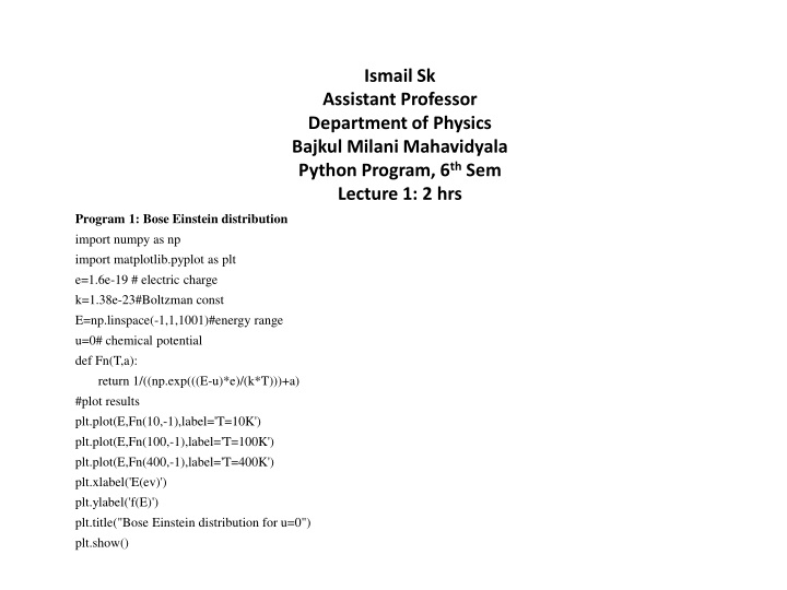
Ismail Sk Assistant Professor Department of Physics Bajkul Milani Mahavidyala Python Program, 6th Sem Lecture 1: 2 hrs Program 1: Bose Einstein distribution import numpy as np import matplotlib.pyplot as plt e=1.6e-19 # electric charge k=1.38e-23#Boltzman const E=np.linspace(-1,1,1001)#energy range u=0# chemical potential def Fn(T,a): return 1/((np.exp(((E-u)*e)/(k*T)))+a) #plot results plt.plot(E,Fn(10,-1),label='T=10K') plt.plot(E,Fn(100,-1),label='T=100K') plt.plot(E,Fn(400,-1),label='T=400K') plt.xlabel('E(ev)') plt.ylabel('f(E)') plt.title("Bose Einstein distribution for u=0") plt.show()
Program 2: Planck law of Radiation import numpy as np import matplotlib.pyplot as plt k=1.38e-23 #boltzman constant h=6.626e-34 c=3e+8 pi=3.14 L0=np.arange(0.1,10,0.005) #wave length in micro m L=L0*1e-6 #wavelength in m def Fn(L,T): a=(8*pi*h*c)/L**5 b=(h*c)/(L*k*T) c1=np.exp(b)-1 d=a/c1 return d #plot results plt.plot(L, Fn(L,500),label='T=500K') plt.plot(L, Fn(L,600),label='T=600K') plt.plot(L, Fn(L,900),label='T=900K') plt.plot(L, Fn(L,1200),label='T=1200K') plt.legend(loc="best" , prop={'size':12}) plt.xlabel("$\lambda$ ") plt.ylabel("U($\lambda $,T )") plt.title("Planck law of Radiation") plt.show()


