Quantifying Performance in Computer Architecture: A Deep Dive into Speedup and Amdahl's Law

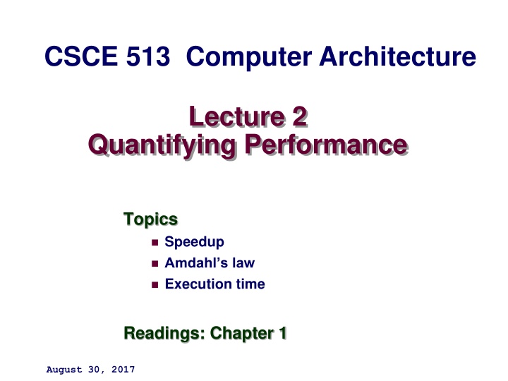
CSCE 513 Computer Architecture Lecture 2 Quantifying Performance Topics Speedup Amdahl s law Execution time Readings: Chapter 1 August 30, 2017

Overview Last Time Overview: Speed-up Power wall, ILP wall, Def Computer Architecture Lecture 1 slides 1-29? to multicore New Syllabus and other course pragmatics Website (not shown) Dates Figure 1.9 Trends: CPUs, Memory, Network, Disk Why geometric mean? Speed-up again Amdahl s Law 2 CSCE 513 Fall 2017

Instruction Set Architecture (ISA) Myopic view of computer architecture ISAs appendices A and K 80x86 ARM MIPS 3 CSCE 513 Fall 2017

MIPS Register Usage Figure 1.4 4 CSCE 513 Fall 2017 Ref. CAAQA

MIPS Instructions Fig 1.5 Data Transfers 5 CSCE 513 Fall 2017 Ref. CAAQA

MIPS Instructions Fig 1.5 Arithmetic/Logical Most significant bit is bit zero; lsb #63 6 CSCE 513 Fall 2017 Ref. CAAQA

MIPS Instructions Fig 1.5 Control Condition Codes set by ALU operations PC Relative branches Jumps JumpAndLink Return address on function call? 7 CSCE 513 Fall 2017 Ref. CAAQA

MIPS Instruction Format (RISC) 8 CSCE 513 Fall 2017 Ref. CAAQA

Fig 1.7 Requirement Challenges for Computer Architects Level of software compatibility Operating system requirements Standards 9 CSCE 513 Fall 2017 Ref. CAAQA

Fig 1.10 Performance over last 25-40 years Processors 10 CSCE 513 Fall 2017 Ref. CAAQA

Fig 1.10 Performance over last 25-40 years Memory 11 CSCE 513 Fall 2017 Ref. CAAQA

Fig 1.10 Performance over last 25-40 years Networks Disk 12 CSCE 513 Fall 2017 Ref. CAAQA

Fig 1.10 Performance over last 25-40 years Processors 13 CSCE 513 Fall 2017 Ref. CAAQA

Quantitative Principles of Design Take advantage of Parallelism Principle of locality Temporal locality Spatial locality Focus on the common case Amdahl s Law 14 CSCE 513 Fall 2017 Ref. CAAQA

Taking Advantage of Parallelism Logic parallelism carry lookahead adder Word parallelism SIMD Instruction pipelining overlap fetch and execute Multithreads executing independent instructions at the same time Speculative execution - 15 CSCE 513 Fall 2017 Ref. CAAQA

Principle of Locality Rule of thumb (Zipf s law?? Not really) A program spends 90% of its execution time in only 10% of the code. So what do you try to optimize? Locality of memory references Temporal locality Spatial locality 16 CSCE 513 Fall 2017

Execution Time of enhanced systems Suppose you have an enhancement or improvement in a design component. The improvement in the performance of the system is limited by the % of the time the enhancement can be used 17 CSCE 513 Fall 2017

Amdahls Law Suppose you have an enhancement or improvement in a design component. The improvement in the performance of the system is limited by the % of the time the enhancement can be used 1 = Speedup overall Frac + [( 1 ) ] Frac enhanced enhanced Speedup enhanced 18 CSCE 513 Fall 2017 Ref. CAAQA

Amdahls with Fractional Use Factor Example:Suppose we are considering an enhancement to a web server. The enhanced CPU is 10 times faster on computation but the same speed on I/O. Suppose also that 60% of the time is waiting on I/O 1 = Speedup overall Frac + [( 1 ) ] Frac enhanced enhanced Speedup enhanced 19 CSCE 513 Fall 2017 Ref. CAAQA

Amdahls Law revisited Speedup = (execution time without enhance.) / (execution time with enhance.) = (time without) / (time with) = Two / Twith Notes 1. The enhancement will be used only a portion of the time. 2. If it will be rarely used then why bother trying to improve it 3. Focus on the improvements that have the highest fraction of use time denoted Fractionenhanced. Note Fractionenhanced is always less than 1. Then 4. 20 CSCE 513 Fall 2017 Ref. CAAQA

Amdahls with Fractional Use Factor Frac = + ExecTime ExecTime * [( 1 ) ] Frac enhanced new old enhanced Speedup enhanced = ( ) /( ) Speedup ExecTime ExecTime overall old new 1 = Frac + [( 1 ) ] Frac enhanced enhanced Speedup enhanced 21 CSCE 513 Fall 2017 Ref. CAAQA

Amdahls with Fractional Use Factor Example:Suppose we are considering an enhancement to a web server. The enhanced CPU is 10 times faster on computation but the same speed on I/O. Suppose also that 60% of the time is waiting on I/O 1 = Speedup Frac overall + [( 1 ) ] Frac enhanced enhanced Speedup enhanced 1 = 4 . ) 4 . + 1 ( 10 1 1 = = 5625 . 1 = + 6 . 04 . Ref. CAAQA 64 . 22 CSCE 513 Fall 2017

Graphics Square Root Enhancement p 40 NewDesign1 FPSQRT 20% speed up FPSQR 10 times NewDesign2 FP improve all FP by 1.6; FP=50% of exec time 23 CSCE 513 Fall 2017 Ref. CAAQA

Geometric Means vs Arithmetic Means 24 CSCE 513 Fall 2017 Ref. CAAQA

Comparing 2 computers Spec_Ratios 25 CSCE 513 Fall 2017 Ref. CAAQA

Performance Measures Response time (latency) -- time between start and completion Throughput (bandwidth) -- rate -- work done per unit time _ _ _ execution time _ without _ enhancemen t = Speedup _ execution time with enhancemen t Processor Speed e.g. 1GHz When does it matter? When does it not? 26 CSCE 513 Fall 2017 Ref. CAAQA

Availability MTTF + = ModuleAvai lability MTTF MTTR 27 CSCE 513 Fall 2017 Ref. CAAQA

MTTF Example 28 CSCE 513 Fall 2017 Ref. CAAQA

Comparing Performance fig 1.15 Comparing three program executing on three machines Computer A Computer B Computer C Program P1 1 10 20 Program P2 1000 100 20 Total Times 1001 110 40 Faster than relationships A is 10 times faster than B on program 1 B is 10 times faster than A on program 2 C is 50 times faster than A on program 2 3 * 2 comparisons (3 choose 2 computers * 2 programs) So what is the relative performance of these machines??? 29 CSCE 513 Fall 2017 Ref. CAAQA

fig 1.15 Total Execution times Comparing three program executing on three machines Computer A Computer B Computer C Program P1 1 10 20 Program P2 1000 100 20 Total times 1001 110 40 So now what is the relative performance of these machines??? B is 1001/110 = 9.1 times as fast as A Arithmetic mean execution time = 30 CSCE 513 Fall 2017 Ref. CAAQA

Weighted Execution Times fig 1.15 Computer A Computer B Computer C Program P1 1 10 20 Program P2 1000 100 20 Program P3 1001 110 40 Now assume that we know that P1 will run 90%, and P2 10% of the time. So now what is the relative performance of these machines??? timeA = .9*1 + .1*1000 = 100.9 timeB = .9*10 +.1*100 = 19 Relative performance A to B = 100.9/19 = 5.31 31 CSCE 513 Fall 2017 Ref. CAAQA

Geometric Means Compare ratios of performance to a standard Using A as the standard program 1 B ratio = 10/1 = 10 C ratio = 20/1 = 20 program 2 Br = 100/1000 = .1 Cr = 20/1000 = .02 B is twice as fast as C using A as the standard Using B as the standard program 1 Ar = 1/10 = .1 Cr = program 2 Br = 1000/100 = 10 Cr = So now compare A and B ratios to each other you get the same 10 and .1, so what? Same ? 32 CSCE 513 Fall 2017 Ref. CAAQA

Geometric Means fig 1.17 Measure performance ratios to a standard machine Normalized to A Normalized to B Normalized to C A B C A B C A B C P1 1.0 10.0 20.0 .1 1.0 2.0 .05 .5 1.0 P2 1.0 .1 .02 10 1.0 .2 50. 5.0 1.0 Arithmetic mean Geometric Mean Total Time 1.0 5.05 10.01 5.05 1.0 1.1 25.03 2.75 1.0 1.0 1.0 .63 1.0 1.0 .63 1.58 1.58 1.0 1.0 .11 .4 9.1 1.0 .36 25.03 2.75 1.0 33 CSCE 513 Fall 2017 Ref. CAAQA

CPU Performance Equation Almost all computers use a clock running at a fixed rate. Clock period e.g. 1GHz = Pr * CPUtime CPUclockCy clesFor ogram ClockCycle Time = Pr / CPUclockCy clesFor ogram ClockRate Instruction Count (IC) CPI = CPUclockCyclesForProgram / InstructionCount CPUtime = IC * ClockCycleTime * CyclesPerInstruction 34 CSCE 513 Fall 2017 Ref. CAAQA

CPU Performance Equation CPUtime = Instructio Pr ns ClockCycle s Seconds Seconds Pr = = CPUtime ogram Instructio n ClockCycle ogram Instruction Count CPI Clock cycle time = n = CPUcycles IC CPI i i 1 i 35 CSCE 513 Fall 2017 Ref. CAAQA

Fallacies and Pitfalls 1. Pitfall: Falling prey to Amdahl s law. 2. Pitfall: A single point of failure. 3. Fallacy: the cost of the processor dominates the cost of the system. 4. Fallacy: Benchmarks remain valid indefinitely. 5. The rated mean time to failure of disks is 1,2000,000 hours or almost 140 years, so disks practically never fail. 6. Fallacy Peak performance tracks observed performance. 7. Pitfall: Fault detection can lower availability. 36 CSCE 513 Fall 2017 Ref. CAAQA

List of Appendices 37 CSCE 513 Fall 2017 Ref. CAAQA

Homework Set #1 Due Friday Sept 6 (Dropbox ) 1. 1.5 2. 1.8 a-d (Change 2015 throughout the question 2017) 3. 1.9 4. 1.18 George K. Zipf (1949) Human Behavior and the Principle of Least Effort. Addison-Wesley 38 CSCE 513 Fall 2017

1.8 [10/ 15/ 15/ 10/ 10] < 1.4, 1.5 > One challenge for architects is that the design created today will require several years of implementation, verification, and testing before appearing on the market. This means that the architect must project what the technology will be like several years in advance. Sometimes, this is difficult to do. a. [10] < 1.4 > According to the trend in device scaling observed by Moore s law, the number of transistors on a chip in 2015 should be how many times the number in 2005? b. b. [15] < 1.5 > The increase in clock rates once mirrored this trend. Had clock rates continued to climb at the same rate as in the 1990s, approximately how fast would clock rates be in 2015? c. c. [15] < 1.5 > At the current rate of increase, what are the clock rates now projected to be in 2015? d. d. [10] < 1.4 > What has limited the rate of growth of the clock rate, and what are architects doing with the extra transistors now to increase performance? Patterson, David A.; Hennessy, John L. (2011-08-01). Computer Architecture: A Quantitative Approach (The Morgan Kaufmann Series in Computer Architecture and Design) (Kindle Locations 2203-2217). Elsevier Science (reference). Kindle Edition. 39 CSCE 513 Fall 2017

Zipf's law Zipf's law states that given some corpus of natural language utterances, the frequency of any word is inversely proportional to its rank in the frequency table. Thus the most frequent word will occur approximately twice as often as the second most frequent word, three times as often as the third most frequent word, etc.: the rank-frequency distribution is an inverse relation. in the Brown Corpus of American English text, "the" is the most frequently occurring word, and by itself accounts for nearly 7% of all word occurrences True to Zipf's Law, the second-place word "of" accounts for slightly over 3.5% of words (36,411 occurrences), followed by "and" (28,852). Only 135 vocabulary items are needed to account for half the Brown Corpus.[4] 40 CSCE 513 Fall 2017

41 CSCE 513 Fall 2017

Stages of Classical 5-stage pipeline Instruction Fetch Cycle IR Mem[PC] NPC PC + 4 Decode A B Imm Regs[rs] sign-extend of Execute . Memory . Write Back . 42 CSCE 513 Fall 2017

Simple RISC Pipeline Clock cycle number (time ) 1 2 3 4 5 6 7 8 9 Instruction IF ID EX MEM WB Instruction n Instruction n+1 IF ID EX MEM WB IF ID EX MEM WB Instruction n+2 IF ID EX MEM WB Instruction n+3 Instruction n+4 IF ID EX MEM WB 43 CSCE 513 Fall 2017

Performance Analysis in Perfect World Assuming S stages in the pipeline. At each cycle a new instruction is initiated. To execute N instructions takes: N cycles to start-up instructions (S-1) cycles to flush the pipeline TotalTime = N + (S-1) Example for S=5 from previous slide N=100 instructions Time to execute in non-pipelined = 100 * 5 = 500 cycles Time to execute in pipelined version = 100 + (5-1) = 104 cycles SpeedUp = 44 CSCE 513 Fall 2017

Implement Pipelines Supp. Fig C.4 45 CSCE 513 Fall 2017

Pipeline Example with a problem (A.5 like) Instruction R1, R2, R3 R4, R1, R5 R6, R1, R7 R8, R1, R9 R10, R1, R11 1 IM 2 ID IM 3 4 5 6 7 8 9 EX ID IM WB DM DM DADD DSUB AND OR XOR EX ID IM WB DM EX ID IM WB DM EX ID WB DM EX WB 46 CSCE 513 Fall 2017

Inserting Pipeline Registers into Data Path fig A.18 0 M u x 1 IF/ID ID/EX EX/MEM MEM/WB Add Add result 4 Add Shift left 2 Read register 1 Instruction Address PC Read data 1 Read register 2 Zero Instruction memory Registers ALU Read data 2 ALU result 0 M u x Read data Write register Address 1 M u x Data memory Write data 1 0 Write data 16 32 Sign extend 47 CSCE 513 Fall 2017

Major Hurdle of Pipelining Consider executing the code below DADD R1, R2, R3 /* R1 R2 + R3 */ DSUB R4, R1, R5 /* R4 R1 + R5 */ AND R6, R1, R7 /* R6 R1 + R7 */ OR R8, R1, R9 /* R8 R1 | R9 */ XOR R10, R1, R11 /* R10 R1 ^ R11 */ 48 CSCE 513 Fall 2017

RISC Pipeline Problems Clock cycle number (time ) Instruction R1, R2, R3 R4, R1, R5 R6, R1, R7 R8, R1, R9 R10, R1, R11 1 IM 2 ID IM 3 4 5 6 7 8 9 EX ID IM WB DM DM DADD DSUB AND OR XOR EX ID IM WB DM EX ID IM WB DM EX ID WB DM EX WB So what s the problem? 49 CSCE 513 Fall 2017

Hazards Data Hazards a data value computed in one stage is not ready when it is needed in another stage of the pipeline Simple Solution: stall until it is ready but we can do better Control or Branch Hazards Structural Hazards arise when resources are not sufficient to completely overlap instruction sequence e.g. two floating point add units then having to do three simultaneously 50 CSCE 513 Fall 2017