Quantile Regression in Microeconometric Modeling
Explore the concept of Quantile Regression in microeconometric modeling through the lens of William Greene's research at the Stern School of Business, New York University. Discover the benefits of using quantile regression, its robustness to extensions, and its ability to provide a complete characterization of the conditional distribution. Delve into topics such as estimated variance, asymptotic theory, bootstrap applications, and the comparison between OLS and Least Absolute Deviations estimators.

Download Presentation

Please find below an Image/Link to download the presentation.
The content on the website is provided AS IS for your information and personal use only. It may not be sold, licensed, or shared on other websites without obtaining consent from the author. If you encounter any issues during the download, it is possible that the publisher has removed the file from their server.
You are allowed to download the files provided on this website for personal or commercial use, subject to the condition that they are used lawfully. All files are the property of their respective owners.
The content on the website is provided AS IS for your information and personal use only. It may not be sold, licensed, or shared on other websites without obtaining consent from the author.
E N D
Presentation Transcript
Microeconometric Microeconometric Modeling Modeling William Greene Stern School of Business New York University [Topic 4-Quantile Regression] 1/9
4. Quantile Regresion [Topic 4-Quantile Regression] 2/9
Quantile Regression Quantile Regression Q(y|x, ) = x, = quantile Estimated by linear programming Q(y|x,.50) = x, .50 median regression Median regression estimated by LAD (estimates same parameters as mean regression if symmetric conditional distribution) Why use quantile (median) regression? Semiparametric Robust to some extensions (heteroscedasticity?) Complete characterization of conditional distribution [Topic 4-Quantile Regression] 3/9
Estimated Variance for Estimated Variance for Quantile Regression Quantile Regression Asymptotic Theory Bootstrap an ideal application [Topic 4-Quantile Regression] 4/9
Asymptotic Theory Based Estimator of Variance of Q-REG x i i i i i y u x x - - x x x = + , ) = , ] = |x Model: , ( Q y | , [ Q u 0 i i i x = Residuals: u y i i i 1 N ( ) 1 1 A C A Asymptotic Variance: 1 N 1 1 B 2 N ] Estimated by i | B = E[f (0) A xx x x i 1 | u u i = 1 i Bandwidth B can be Silverman's Rule of Thumb: 1.06 Min s N ( |.75) ( |.25) Q u Q u i i , u .2 1.349 (1- ) N ] Estimated by (1- ) [ C = xx X X E ( ) 1 For =.5 and normally distributed u, this all simplifies to 2 X X . us 2 But, this is an ideal application for bootstrapping . [Topic 4-Quantile Regression] 5/9
= .25 = .50 = .75 [Topic 4-Quantile Regression] 6/9
OLS vs. Least Absolute Deviations OLS vs. Least Absolute Deviations ---------------------------------------------------------------------- Least absolute deviations estimator............... Residuals Sum of squares = 1537.58603 Standard error of e = 6.82594 Fit R-squared = .98284 Adjusted R-squared = .98180 Sum of absolute deviations = 189.3973484 --------+------------------------------------------------------------- Variable| Coefficient Standard Error b/St.Er. P[|Z|>z] Mean of X --------+------------------------------------------------------------- |Covariance matrix based on 50 replications. Constant| -84.0258*** 16.08614 -5.223 .0000 Y| .03784*** .00271 13.952 .0000 9232.86 PG| -17.0990*** 4.37160 -3.911 .0001 2.31661 --------+------------------------------------------------------------- Ordinary least squares regression ............ Residuals Sum of squares = 1472.79834 Standard error of e = 6.68059 Standard errors are based on Fit R-squared = .98356 50 bootstrap replications Adjusted R-squared = .98256 --------+------------------------------------------------------------- Variable| Coefficient Standard Error t-ratio P[|T|>t] Mean of X --------+------------------------------------------------------------- Constant| -79.7535*** 8.67255 -9.196 .0000 Y| .03692*** .00132 28.022 .0000 9232.86 PG| -15.1224*** 1.88034 -8.042 .0000 2.31661 --------+------------------------------------------------------------- [Topic 4-Quantile Regression] 7/9