Quantitative Approaches to Forecasting: Time Series Analysis
Quantitative forecasting methods involve analyzing historical data of time series to make predictions. Explore the components of a time series, measures of forecast accuracy, and the use of smoothing methods. Understand the trends, seasonal patterns, and irregularities in time series data. Learn how to minimize forecast errors and enhance accuracy in forecasting models.

Uploaded on Feb 18, 2025 | 1 Views
Download Presentation

Please find below an Image/Link to download the presentation.
The content on the website is provided AS IS for your information and personal use only. It may not be sold, licensed, or shared on other websites without obtaining consent from the author.If you encounter any issues during the download, it is possible that the publisher has removed the file from their server.
You are allowed to download the files provided on this website for personal or commercial use, subject to the condition that they are used lawfully. All files are the property of their respective owners.
The content on the website is provided AS IS for your information and personal use only. It may not be sold, licensed, or shared on other websites without obtaining consent from the author.
E N D
Presentation Transcript
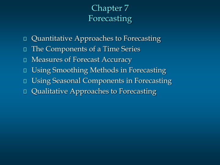
Chapter 7 Forecasting Quantitative Approaches to Forecasting The Components of a Time Series Measures of Forecast Accuracy Using Smoothing Methods in Forecasting Using Seasonal Components in Forecasting Qualitative Approaches to Forecasting
Quantitative Approaches to Forecasting Quantitative methods are based on an analysis of historical data concerning one or more time series. A time series is a set of observations measured at successive points in time or over successive periods of time. If the historical data used are restricted to past values of the series that we are trying to forecast, the procedure is called a time series method. If the historical data used involve other time series that are believed to be related to the time series that we are trying to forecast, the procedure is called a causal method.
Time Series Trend component Demand for product or service Seasonal peaks Actual demand Average demand over four years Random variation | 1 | 2 | 3 | 4 Year
Components of a Time Series The trend component accounts for the gradual shifting of the time series over a long period of time. Any regular pattern of sequences of values above and below the trend line is attributable to the cyclical component of the series. 0 5 10 15 20
Components of a Time Series The seasonal component of the series accounts for regular patterns of variability within certain time periods, such as over a year. The irregular component of the series is caused by short-term, unanticipated and non-recurring factors that affect the values of the time series. One cannot attempt to predict its impact on the time series in advance. M T W T F
Measures of Forecast Accuracy Mean Squared Error The average of the squared forecast errors for the historical data is calculated. The forecasting method or parameter(s) which minimize this mean squared error is then selected. Mean Absolute Deviation The mean of the absolute values of all forecast errors is calculated, and the forecasting method or parameter(s) which minimize this measure is selected. The mean absolute deviation measure is less sensitive to individual large forecast errors than the mean squared error measure.
Smoothing Methods In cases in which the time series is fairly stable and has no significant trend, seasonal, or cyclical effects, one can use smoothing methods to average out the irregular components of the time series. Four common smoothing methods are: Moving averages Centered moving averages Weighted moving averages
Smoothing Methods Moving Average Method The moving average method consists of computing an average of the most recent n data values for the series and using this average for forecasting the value of the time series for the next period.
Example: Rosco Drugs Sales of Comfort brand headache medicine for the past ten weeks at Rosco Drugs are shown on the next slide. If Rosco Drugs uses a 3-period moving average to forecast sales, what is the forecast for Week 11?
Example: Rosco Drugs Past Sales 1 110 6 120 2 115 7 130 3 125 8 115 4 120 9 110 5 125 10 130 WeekSalesWeekSales
Example: Rosco Drugs Excel Spreadsheet Showing Input Data A B C 1 2 3 4 5 6 7 8 9 Robert's Drugs Week (t) 1 2 3 4 5 6 7 8 9 10 Salest 110 115 125 120 125 120 130 115 110 130 Forect+1 10 11 12 13
Example: Rosco Drugs Steps to Moving Average Using Excel Step 1: Select the Tools pull-down menu. Step 2: Select the Data Analysis option. Step 3: When the Data Analysis Tools dialog appears, choose Moving Average. Step 4: When the Moving Average dialog box appears: Enter B4:B13 in the Input Range box. Enter 3 in the Interval box. Enter C4 in the Output Range box. Select OK.
Example: Rosco Drugs Spreadsheet Showing Results Using n = 3 A B C 1 2 3 4 5 6 7 8 9 Robert's Drugs Week (t) 1 2 3 4 5 6 7 8 9 10 Salest 110 115 125 120 125 120 130 115 110 130 Forect+1 #N/A #N/A #N/A 116.7 120.0 123.3 121.7 125.0 121.7 118.3 10 11 12 13
Smoothing Methods Centered Moving Average Method The centered moving average method consists of computing an average of n periods' data and associating it with the midpoint of the periods. For example, the average for periods 5, 6, and 7 is associated with period 6. This methodology is useful in the process of computing season indexes.
Example: Rosco Drugs Spreadsheet Showing Results Using n = 3 A B C 1 2 3 4 5 6 7 8 9 Robert's Drugs Week (t) 1 2 3 4 5 6 7 8 9 10 Salest 110 115 125 120 125 120 130 115 110 130 Forect+1 #N/A 116.7 120.0 123.3 121.7 125.0 121.7 118.6 118.3 #N/A 10 11 12 13
Trend Projection Using the method of least squares, the formula for the trend projection is: Tt= b0 + b1t. where: Tt = trend forecast for time period t b1 = slope of the trend line b0 = trend line projection for time 0 b1 = n tYt - t Yt n t 2 - ( t )2 = Y b t b 0 1 where: Yt = observed value of the time series at time period t = average of the observed values for Yt = average time period for the n observations t Y
Example: Augers Plumbing Service The number of plumbing repair jobs performed by Auger's Plumbing Service in each of the last nine months is listed on the next slide. Forecast the number of repair jobs Auger's will perform in December using the least squares method.
Example: Augers Plumbing Service Month Jobs Month Jobs Month Jobs March 353 June 374 September 399 April 387 July 396 October 412 May 342 August 409 November 408
Example: Augers Plumbing Service Trend Projection (month) tYttYtt 2 (Mar.) 1 353 353 1 (Apr.) 2 387 774 4 (May) 3 342 1026 9 (June) 4 374 1496 16 (July) 5 396 1980 25 (Aug.) 6 409 2454 36 (Sep.) 7 399 2793 49 (Oct.) 8 412 3296 64 (Nov.) 9 408 3672 81 Sum 45 3480 17844 285
Example: Augers Plumbing Service Trend Projection (continued) = 45/9 = 5 = 3480/9 = 386.667 t Y n tYt - t Yt (9)(17844) - (45)(3480) b1 = = n t 2 - ( t)2 (9)(285) - (45)2 = 386.667 - 7.4(5) = 349.667 0 1 b Y b t = = 7.4 T10 = 349.667 + (7.4)(10) = 423.667
Example: Augers Plumbing Service Excel Spreadsheet Showing Input Data A B C 1 2 3 4 5 6 7 8 9 Auger's Plumbing Service Month 1 2 3 4 5 6 7 8 9 Calls 353 387 342 374 396 409 399 412 408 10 11 12 13
Example: Augers Plumbing Service Steps to Trend Projection Using Excel Step 1: Select an empty cell (B13) in the worksheet. Step 2: Select the Insert pull-down menu. Step 3: Choose the Function option. Step 4: When the Paste Function dialog box appears: Choose Statistical in Function Category box. Choose Forecast in the Function Name box. Select OK. more . . . . . . .
Example: Augers Plumbing Service Steps to Trend Projecting Using Excel (continued) Step 5: When the Forecast dialog box appears: Enter 10 in the x box (for month 10). Enter B4:B12 in the Known y s box. Enter A4:A12 in the Known x s box. Select OK.
Example: Augers Plumbing Service Spreadsheet with Trend Projection for Month 10 A B C 1 2 3 4 5 6 7 8 9 Auger's Plumbing Service Month 1 2 3 4 5 6 7 8 9 10 Calls 353 387 342 374 396 409 399 412 408 423.667 Projected 10 11 12 13
Forecasting with Trend and Seasonal Components Steps of Multiplicative Time Series Model 1. Calculate the centered moving averages (CMAs). 2. Center the CMAs on integer-valued periods. 3. Determine the seasonal and irregular factors (StIt ). 4. Determine the average seasonal factors. 5. Scale the seasonal factors (St ). 6. Determine the deseasonalized data. 7. Determine a trend line of the deseasonalized data. 8. Determine the deseasonalized predictions. 9. Take into account the seasonality.
Example: Terrys Tie Shop Business at Terry's Tie Shop can be viewed as falling into three distinct seasons: (1) Christmas (November-December); (2) Father's Day (late May - mid-June); and (3) all other times. Average weekly sales ($) during each of the three seasons during the past four years are shown on the next slide. Determine a forecast for the average weekly sales in year 5 for each of the three seasons.
Example: Terrys Tie Shop Past Sales ($) Season 1 2 3 4 1 1856 1995 2241 2280 2 2012 2168 2306 2408 3 985 1072 1105 1120 Year
Example: Terrys Tie Shop Year Season Sales (Yt) Average StItStYt/St 1 1 1856 1.178 1576 2 2012 1617.67 1.244 1.236 1628 3 985 1664.00 .592 .586 1681 2 1 1995 1716.00 1.163 1.178 1694 2 2168 1745.00 1.242 1.236 1754 3 1072 1827.00 .587 .586 1829 3 1 2241 1873.00 1.196 1.178 1902 2 2306 1884.00 1.224 1.236 1866 3 1105 1897.00 .582 .586 1886 4 1 2280 1931.00 1.181 1.178 1935 2 2408 1936.00 1.244 1.236 1948 3 1120 .586 1911 Dollar Moving Scaled
Example: Terrys Tie Shop 1. Calculate the centered moving averages. There are three distinct seasons in each year. Hence, take a three-season moving average to eliminate seasonal and irregular factors. For example: 1st MA = (1856 + 2012 + 985)/3 = 1617.67 2nd MA = (2012 + 985 + 1995)/3 = 1664.00 etc.
Example: Terrys Tie Shop 2. Center the CMAs on integer-valued periods. The first moving average computed in step 1 (1617.67) will be centered on season 2 of year 1. Note that the moving averages from step 1 center themselves on integer-valued periods because n is an odd number.
Example: Terrys Tie Shop 3. Determine the seasonal & irregular factors (St It ). Isolate the trend and cyclical components. For each period t, this is given by: St It = Yt /(Moving Average for period t )
Example: Terrys Tie Shop 4. Determine the average seasonal factors. Averaging all St Itvalues corresponding to that season: Season 1: (1.163 + 1.196 + 1.181) /3 = 1.180 Season 2: (1.244 + 1.242 + 1.224 + 1.244) /4 = 1.238 Season 3: (.592 + .587 + .582) /3 = .587
Example: Terrys Tie Shop 5. Scale the seasonal factors (St ). Average the seasonal factors = (1.180 + 1.238 + .587)/3 = 1.002. Then, divide each seasonal factor by the average of the seasonal factors. Season 1: 1.180/1.002 = 1.178 Season 2: 1.238/1.002 = 1.236 Season 3: .587/1.002 = .586 Total = 3.000
Example: Terrys Tie Shop 6. Determine the deseasonalized data. Divide the data point values, Yt , by St . 7. Determine a trend line of the deseasonalized data. Using the least squares method for t = 1, 2, ..., 12, gives: Tt = 1580.11 + 33.96t
Example: Terrys Tie Shop 8. Determine the deseasonalized predictions. Substitute t = 13, 14, and 15 into the least squares equation: T13 = 1580.11 + (33.96)(13) = 2022 T14 = 1580.11 + (33.96)(14) = 2056 T15 = 1580.11 + (33.96)(15) = 2090
Example: Terrys Tie Shop 9. Take into account the seasonality. Multiply each deseasonalized prediction by its seasonal factor to give the following forecasts for year 5: 2382 2541 1225 Season 1: (1.178)(2022) = Season 2: (1.236)(2056) = Season 3: ( .586)(2090) =
Qualitative Approaches to Forecasting Delphi Approach A panel of experts, each of whom is physically separated from the others and is anonymous, is asked to respond to a sequential series of questionnaires. After each questionnaire, the responses are tabulated and the information and opinions of the entire group are made known to each of the other panel members so that they may revise their previous forecast response. The process continues until some degree of consensus is achieved.
Qualitative Approaches to Forecasting Scenario Writing Scenario writing consists of developing a conceptual scenario of the future based on a well defined set of assumptions. After several different scenarios have been developed, the decision maker determines which is most likely to occur in the future and makes decisions accordingly.
Qualitative Approaches to Forecasting Subjective or Interactive Approaches These techniques are often used by committees or panels seeking to develop new ideas or solve complex problems. They often involve "brainstorming sessions". It is important in such sessions that any ideas or opinions be permitted to be presented without regard to its relevancy and without fear of criticism.