Random Variables and Expectations in Engineering Applications
This content discusses expectations of random variables and functions of random variables in ECE 313 Probability with Engineering Applications. Topics cover important distributions such as hypo-exponential, Erlang, and hyper-exponential, along with the calculation of expectations for various random variables. Examples include discrete random variables and Bernoulli random variables.

Download Presentation

Please find below an Image/Link to download the presentation.
The content on the website is provided AS IS for your information and personal use only. It may not be sold, licensed, or shared on other websites without obtaining consent from the author.If you encounter any issues during the download, it is possible that the publisher has removed the file from their server.
You are allowed to download the files provided on this website for personal or commercial use, subject to the condition that they are used lawfully. All files are the property of their respective owners.
The content on the website is provided AS IS for your information and personal use only. It may not be sold, licensed, or shared on other websites without obtaining consent from the author.
E N D
Presentation Transcript
Expectations of Random Variables, Functions of Random Variables ECE 313 Probability with Engineering Applications Lecture 16 Ravi K. Iyer Dept. of Electrical and Computer Engineering University of Illinois at Urbana Champaign Iyer - Lecture 16 ECE 313 Spring 2017
Todays Topics review hypo, Erlang and Hyper Exponential distributions Expectations Expectations of important random variables - Short quiz Announcements Homework 7. Based on your Midterm exam, individual problems are assigned to you to solve. Checkout Compass. Midterm regrades. Submit today a brief concept quiz Mini Project 2 grades posted this week Final project dates will be announced soon Iyer - Lecture 16 ECE 313 Spring 2017
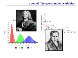
Summary of important distributions 1 2 2 1 Hypo exponential (two-phase) (e 1t e 2t), t 0 f(t) = 2 1/?? 1/?? ? ?/? ? K-stage Erlang ?/?2 Gamma ??2 ?? Hyper exponential ??/?? ? Iyer - Lecture 16 ECE 313 Spring 2017
Exponential & related Distributions Iyer - Lecture 16 ECE 313 Spring 2017
Expectation of a Random Variable The Discrete Case: If X is a discrete random variable having a probability mass function p(x), then the expected value of X is defined by : p x = [ ] ( ) E X xp x ( ) 0 x The expected value of X is a weighted average of the possible values that X can take on, each value being weighted by the probability that X assumes that value. For example, if the probability mass function of X is given by 1 ) 1 ( p = = ) 2 ( p then 2 1 1 3 = + = [ ] 1 2 E x 2 2 2 is just an ordinary average of the two possible values 1 and 2 that X can assume. Iyer - Lecture 16 ECE 313 Spring 2017
Expectation of a Random Variable (Cont.) Assume 1 2 = = ) 1 ( p , ) 2 ( p 3 1 3 2 5 Then = + = [ ] 1 2 E X 3 3 3 is a weighted average of the two possible values 1 and 2 where the value 2 is given twice as much weight as the value 1 since p(2) = 2p(1). Find E[X] where X is the outcome when we roll a fair die. Solution: Since p p p p ) 4 ( ) 3 ( ) 2 ( ) 1 ( = = = 1 = = = ) 5 ( ) 6 ( , p p we obtain 6 Iyer - Lecture 16 ECE 313 Spring 2017
Expectation of a Random Variable (Cont.) Expectation of a Bernoulli Random Variable: Calculate E[X] when X is a Bernoulli random variable with parameter p. = ] = ( 1 ) 0 ( 1 , ) 1 ( p p p p Since: We have: = + = [ 1 ( 0 ) ) E X p p p Iyer - Lecture 16 ECE 313 Spring 2017
Expectation of a Random Variable (Cont.) Expectation of a Binomial Random Variable: Calculate E[X] when X is a binomially distributed with parameters n and p. Let k = i 1.. Iyer - Lecture 16 ECE 313 Spring 2017
Expectation of a Random Variable (Cont.) Expectation of a Geometric Random Variable: Calculate the expectation of a geometric random variable having parameter p. We have: = = 1 d = = n [ ] ( ) E X p q 1 n [ ] 1 ( ) E X np p dq 1 n n d = = n p q = 1 = 1 n p nq dq 1 n 1 n d q = where q p = p 1 dq q p = 2 1 ( ) q The expected number of independent trials we need to perform until we get our first success equals the reciprocal of the probability that any one trial results in a success. 1 = p Iyer - Lecture 16 ECE 313 Spring 2017
Expectation of a Random Variable (Cont.) Expectation of a Poisson Random Variable: Calculate E[X] if X is a Poisson random variable with parameter . where we have used the identity: = 0 / k = k ! k e Iyer - Lecture 16 ECE 313 Spring 2017
The Continuous Case The expected value of a continuous random variable: If X is a continuous random variable having a density function f (x), then the expected value of X is defined by: = [ ] ( ) E X xf x dx Example: Expectation of a Uniform Random Variable, Calculate the expectation of a random variable uniformly distributed over ( , ) x = [ ] E X dx 2 2 = + ( 2 ) = 2 Iyer - Lecture 16 ECE 313 Spring 2017
The Continuous Case (Cont.) Expectation of an Exponential Random Variable: Let X be exponentially distributed with parameter . Calculate E[X]. Integrating by parts: Iyer - Lecture 16 ECE 313 Spring 2017
The Continuous Case Cont d Expectation of a Normal Random Variable): X is normally distributed with parameters and 2: X E 2 1 22 / 2 = ( ) x [ ] xe dx Writing x as (x- ) + yields 1 1 2 2 2 2 = + ( ) / 2 ( ) / 2 x x [ ] ( ) E X x e dx e dx 2 2 Letting y= x- leads to 1 22 / 2 = + y [ ] ( dx ) E X ye dy f x 2 Where f(x) is the normal density. By symmetry, the first integral must be 0, and so = = [ ] ( dx ) E X f x Iyer - Lecture 16 ECE 313 Spring 2017
Example: Searching a table sequentially Consider the problem of searching for a specific name in a table of names. A simple method is to scan the table sequentially, starting from one end, until we either find the name or reach the other end, indicating that the required name is missing from the table. The following is a C program fragment for sequential search: Iyer - Lecture 16 ECE 313 Spring 2017
Example Cont d In order to analyze the time required for sequential search, let X be the discrete random variable denoting the number of comparisons myName Table[I] made. The set of all possible values of X is {1,2, ,n+1}, and X=n+1 for unsuccessful searches. More interesting to consider a random variable Y that denotes the number of comparisons for a successful search. The set of all possible values of Y is {1,2, ,n}. To compute the average search time for a successful search, we must specify the pmf of Y. In the absence of any specific information, let us assume that Y is uniform over its range: 1 ) ( n i n ) 1 ( 1 ) ( ] [ 1 = n i = , 1 . pY i + ) 1 + Then ( n n n n = = = . E Y i p i 2 2 Y Thus, on the average, approximately half the table needs to be searched Iyer - Lecture 16 ECE 313 Spring 2017
Example Table ordered by non increasing access probabilities If idenotes the access probability for name Table[i], then the average successful search time is E[Y] is minimized when names in the table are in the order of non-increasing access probabilities; that is, 1 2 n. c = , 1 , i n 1 i = n i 1= 1 Where the constant c is determined from the normalization requirement 1 1 n 1 1 = = , c Thus, + 1 i ln( ) H n C = n 1 i = n = / 1 ( ) H i Where Hnis the partial sum of a harmonic series; that is: and C(=0.577) is the Euler Constant. Now, if the names in the table are ordered as above, then the average search time is i Y E i n i = = 1 1 n 1 i 1 n n n n ) = = = [ ] 1 i + ln( H H n C n Which is considerably less than the previous value (n+1)/2, for large n Iyer - Lecture 16 ECE 313 Spring 2017
Iyer - Lecture 16 ECE 313 Spring 2017
Moments of a Distribution Let X be a random variable, and define another random variable Y as a function of X so that To compute E[Y] ). (X Y = (provided the sum or the integral on the right-hand side is absolutely convergent). A special case of interest is the power function For k=1,2,3, , is known as the kth moment of the random variable X. Note that the first moment is the ordinary expectation or the mean of X. We define the kth central moment, of the random variable X by k X = ) k ( X k [ ] E X [X ] E 2 Known as the variance of X, Var[X], often denoted by i (xi-E[X])2p(xi) if Xisdiscrete Var[X]=s2= (x-E[X])2f(x)dx if Xiscontinuous - It is clear that Var[X] is always a nonnegative number. Iyer - Lecture 16 ECE 313 Spring 2017
Variance: 2ndCentral Moment We define the kth central moment, of the random variable X by [( k X E = k k [ ]) ] E X = 2 2 2 [( [ ]) ] E X E X known as the variance of X, Var[X], often denoted by Definition (Variance). The variance of a random variable X is i (xi-E[X])2p(xi) if Xisdiscrete Var[X]=s2= (x-E[X])2f(x)dx if Xiscontinuous - It is clear that Var[X] is always a nonnegative number. Iyer - Lecture 16 ECE 313 Spring 2017
Functions of a Random Variable = As an example, X could denote the measurement X = 2 ( ) Y X Let error in a certain physical experiment and Y would then be the square of the error (e.g. method of least squares). Note that = ) ( ) y Y P y F ( ) 0 for . 0 For , 0 y y y Y = ( F Y = 2 ( ) P X y = ( ) P y X y = ( ) ( ), F y F y X X differenti by and ation the density of is Y 1 + [ ( ) ( )], , 0 f y f y y = X X ( ) f y 2 y Y , 0 . otherwise Iyer - Lecture 16 ECE 313 Spring 2017
Functions of a Random Variable (cont.) Let X have the standard normal distribution [N(0,1)] so that 1 ) ( e x f X 2 = / 2 x , . x 2 Then 1 1 1 , 0 + y / 2 / 2 y y e e = ( ) , f y 2 2 2 y Y , 0 y , 0 or , 0 y 1 / 2 y , e = ( ) f y . 0 y 2 y Y , 0 This is a chi-squared distribution with one degree of freedom Iyer - Lecture 16 ECE 313 Spring 2017
Functions of a Random Variable (cont.) Generating Exponential Random Numbers Let X be uniformly distributed on (0,1). We show that has an exponential distribution with parameter Note: Y is a nonnegative random variable: = 1 ln( 1 ) Y X . 0 FY(y)=0fory 0. This fact can be used in a distribution-driven simulation. In simulation programs it is important to be able to generate values of variables with known distribution functions. Such values are known as random deviates or random variates. Most computer systems provide built-in functions to generate random deviates from the uniform distribution over (0,1), say u. Such random deviates are called random numbers. Iyer - Lecture 16 ECE 313 Spring 2017
Expectation of a Function of a Random Variable Given a random variable X and its probability distribution or its pmf/pdf We are interested in calculating not the expected value of X, but the expected value of some function of X, say, g(X). One way: since g(X) is itself a random variable, it must have a probability distribution, which should be computable from a knowledge of the distribution of X. Once we have obtained the distribution of g(X), we can then compute E[g(X)] by the definition of the expectation. Example 1: Suppose X has the following probability mass function: ) 2 ( , 5 . 0 ) 1 ( , 2 . 0 ) 0 ( = = = p p p 3 . 0 Calculate E[X2]. Letting Y=X2,we have that Y is a random variable that can take on one of the values, 02, 12, 22with respective probabilities Hence, = E X E pY(1)= P{Y =12}= 0.5 pY(2)= P{Y =22}=0.3 pY(0)= P{Y =02}=0.2 = ) 5 . 0 ( 1 + ) 3 . 0 ( 4 + 7 . 1 = 2 [ ] [ ] ) 2 . 0 ( 0 Y Note that = . 1 = 2 2 1. 7 [ ] [ ] 21 E X E X Iyer - Lecture 16 ECE 313 Spring 2017
Expectation of a Function of a Random Variable (cont.) Proposition 2: (a) If X is a discrete random variable with probability mass function p(x), then for any real-valued function g, 0 ) ( : x p x = [ ( )] ( ) ( ) E g X g x p x (b) if X is a continuous random variable with probability density function f(x), then for any real-valued function g: dx x f x g X g E = [ ( )] ( ) ( ) Example 3, Applying the proposition to Example 1 yields ) 5 . 0 )( 1 ( ) 2 . 0 ( 0 ] [ + + = X E 7 . 1 = 2 2 2 2 2 ( ) 3 . 0 )( Example 4, Applying the proposition to Example 2 yields 1 3 3 = = ) 1 [ ] dx (since 1 0 E X x f(x) , x 0 1 = 4 Iyer - Lecture 16 ECE 313 Spring 2017
Corollary + = + [ ] [ ] E aX b aE X b If a and b are constants, then The discrete case: E ( + = + [ ] ( ) ( ) aX b ax 0 b p x : ) x p x ( ( = + ( ) ( ) a xp ] x b p 0 x : ) 0 : ) x p [ x x p x = + aE X b The continuous case: + = + [ ] ( ) ( ) E aX b ax b f x dx = + ( ) ( ) a xf x dx b f x dx = + [ ] aE X b Iyer - Lecture 16 ECE 313 Spring 2017
Moments The expected value of a random variable X, E[X], is also referred to as the mean or the first moment of X. n The quantity is called the nth moment of X. We have: xnp(x), x:p(x)>0 [ ], 1 E X n if X is discrete E[Xn]= xnf(x)dx, if X is continuous - Another quantity of interest is the variance of a random variable X, denoted by Var(X), which is defined by: = 2 ( ) [( [ ]) ] Var X E X E X Iyer - Lecture 16 ECE 313 Spring 2017


")
")
")
")
")

")


")
")