Rational Transforms & Partial Fractions in Inverse Laplace Transform
Consider finding the inverse Laplace transform using rational transforms & partial fractions. Learn the methods for distinct roots, complex poles, & more with examples. Use MATLAB for computations.

Download Presentation

Please find below an Image/Link to download the presentation.
The content on the website is provided AS IS for your information and personal use only. It may not be sold, licensed, or shared on other websites without obtaining consent from the author.If you encounter any issues during the download, it is possible that the publisher has removed the file from their server.
You are allowed to download the files provided on this website for personal or commercial use, subject to the condition that they are used lawfully. All files are the property of their respective owners.
The content on the website is provided AS IS for your information and personal use only. It may not be sold, licensed, or shared on other websites without obtaining consent from the author.
E N D
Presentation Transcript
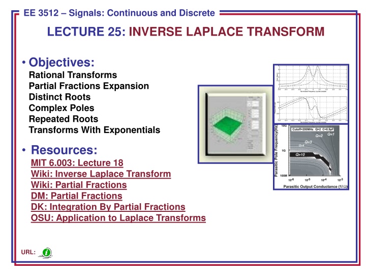
ECE 8443 Pattern Recognition EE 3512 Signals: Continuous and Discrete LECTURE 25: INVERSE LAPLACE TRANSFORM Objectives: Rational Transforms Partial Fractions Expansion Distinct Roots Complex Poles Repeated Roots Transforms With Exponentials Resources: MIT 6.003: Lecture 18 Wiki: Inverse Laplace Transform Wiki: Partial Fractions DM: Partial Fractions DK: Integration By Partial Fractions OSU: Application to Laplace Transforms URL:
Rational Transforms Consider the problem of finding the inverse Laplace transform for: s b s b s b b s A + + + ... ) ( 2 1 0 + + + 2 M ... 2 ( ) B s = = 0 1 2 M ( ) X s N a a s a s a s N where {ai} and {bi} are real numbers, and M and N are positive integers. One straightforward approach is to factor B(s) into a sum of simpler terms whose Laplace transforms can be easily computed (or located in a table of transform pairs). The method of Partial Fractions is one approach: c p s p s p s a ) )...( )( ( 2 1 + + + 2 M ... b b s b s b s c c = = + + + 0 1 2 M N 1 2 ( ) ... X s s p s p s p 1 2 N N N The details of the expansion depends on the properties of A(s). For example, the presence of repeated roots slightly complicates things. Fortunately, MATLAB can be used to find the roots of the polynomial: 4 6 4 ) ( + + + = s s s s A 3 2 A = [1 4 6 4] p = roots(A) p = -2 -1.0000 + 1.0000i -1.0000 1.0000i = + + + + ( ) ( 2 )( 1 )( 1 ) A s s s j s j EE 3512: Lecture 25, Slide 1
Distinct Roots: Method of Residues Suppose there are distinct or non-repeated roots: pi pj when i j. c p s p s N ,..., 2 , 1 , )] ( ) [( = = = c c = + + + N 1 2 ( ) ... X s s p 1 2 c s p X s i N i i s ip The constants, ci, are called residues, and this method of computation is called the residue method. The constant ci is real if the corresponding pole is real. If two poles appear as complex conjugate pairs, the ci must also appear in complex conjugate pairs. Once the partial fractions expansion is completed, the inverse Laplace transform can be easily found as: 0 ... ) ( 2 1 + + + = t e c e c e c t x N p t p t p t N 1 2 MATLAB can be used to find poles as residues: num = [bM bM-1 b1 b0] den = [aN aN-1 a1 a0] [r,p] = residue(num, den) Example: + s + c c c c c c 2 2 2 s s s = = = + + = + + 3 3 1 2 1 2 ( ) X s + + ) 1 ) 3 + + + + 3 ( 1 )( ) 3 0 ( ( 1 3 s s s s s s s s 4 3 s s EE 3512: Lecture 25, Slide 2
Distinct Roots (Cont.) Example: + s c c c 2 2 s = = + + 3 1 2 ( ) X s + + + + 3 1 3 s s s 4 3 s s + 2 s 2 s = = = [ ( )] c sX s = 1 0 s + + ( 1 )( ) 3 3 s = 0 s + 2 1 s = ) 1 + = = [( ( )] c s X s = 2 1 s + ( ) 3 2 s s = 1 s + 2 1 s = + = = [( ) 3 ( )] c s X s = 3 3 s ) 1 + ( 6 s s = 3 s 2 ( ) 3 / s ( / 1 + s ) 2 ( / 1 + s ) 6 2 1 1 = + + = 3 t t ( ) ( ) , 0 X s x t e e t 1 3 3 2 6 This can be checked with MATLAB: num = [1 2] den = [1 4 3 0] [r,p] = residue(num, den) r = p = -0.1667 -3 -0.5000 -1 0.6667 0 EE 3512: Lecture 25, Slide 3
Distinct Complex Poles Recall if all coefficients of the denominator are real, then the polynomial must have a combination of real and/or complex conjugate poles. We can factor this polynomial into the following form: c p s 1 1 = + j p c c 1 = + + + N 1 1 ( ) ... where X s = j p s p s p 1 N The inverse transform is given by: p t p e c e c t x + = ) ( 1 1 + + = + + + p t p t t t ... 2 cos( ) ... c e c e t c c e N N 1 1 1 1 N N How can this be visualized in the s-plane? (Hint: frequency and bandwidth) Example: s + 2 c c c 2 1 s s s = = + + 3 1 1 ( ) X s + ) 1 + + + 3 2 ( 1 ) ( 1 ) ( s j s j s 3 4 2 s + s 2 2 j 1 3 s s = + = = + [( 1 ) ( )] 2 c s j X s j = + 1 1 s j + + ) 1 + ( 1 )( 2 s = + 1 s j j + 2 2 1 s s = ) 1 + = = [( ( )] 4 c s X s = 3 1 s + + + ( 1 )( 1 ) s s j = 1 s = = = = 5 / 2 126 87 . Re{ } 1 c c p 1 1 1 = + + t t ( ) 5 cos( 126 87 . ) 4 , 0 x t e t e t EE 3512: Lecture 25, Slide 4
Repeated Poles If the denominator has repeated poles, the expansion is of the form: c p s p s ( ) ( 1 1 c c c c = + + + + + + + + N 1 2 1 r p r ( ) ... ... ... X s 2 r s p s p ) s + 1 r N 1 The residues for the nonrepeated poles are calculated the same as before: r r i s X p s c ip s i i ..., , 2 , 1 , )] ( ) [( + + = = = N The residues for the repeated poles are calculated by: )] ( ) [( 1 1 = = d i r c s p X s r s p i 1 = = r [ [( ) ( )]] , , 1 , 2 ..., 1 c s p X s i r = 1 r i s p i ! ds 1 If the poles are all real, the inverse can be compactly written using: N e N ) ( )! 1 ( + 1 1 t at N s a Repeated complex poles and complex conjugate poles can also be dealt with by combining the complex conjugate poles into one quadratic term, and solving for the residues by equating terms of a polynomial: + + c c cs d cs d = + + = + = + 1 1 ( ) ... ... ... X s 2 ( )( ) s p s p s p s p + 2 s p 1 1 1 1 1 EE 3512: Lecture 25, Slide 5
Repeated Poles (Cont.) Example: s c c c 5 1 s = = + + 3 1 1 ( ) X s + + 3 2 1 2 s s 3 2 ( ) 1 s s 5 s 1 d d s = ) 1 + = 2 ( ( ) c s X s 1 2 ds ds = 1 s = 1 s 1 1 9 = + = = ) 5 ( 5 ( 1 )( ) 1 s ( ) 2 2 2 s ( ) 2 s 2 s = 1 s = 1 s 5 s 1 s = ) 1 + = = 2 ( ( ) 2 c s X s = 2 1 s 2 = 1 s = = 2 ( ) 2 ( ) 1 c s X s = 3 2 s Compute the inverse of each term individually and sum them: = + + 2 t t t ( ) 2 , 0 x t e te e t This can be easily checked using MATLAB. EE 3512: Lecture 25, Slide 6
Numerator Has A Larger Order (M N) What if the numerator has a degree larger than the denominator? The polynomials can be decomposed using long division: ... ) ( 2 1 0 s a s a a s A + + + + + 2 M b b s b s b s ( ) ( ) B s R s = = = + 0 1 2 M ( ) ( ) X s Q s + 2 N ( ) A s ... a s N The inverse transform of Q(s) is computing using the transform pair: d N N N = ( ) , , 1 , 2 ... t s N dt Example: + 3 2 4 20 2 12 s s s s = = + ( ) 4 X s s + + 2 4 2 s s 4 2 s d = + ( ) ( ) 4 ( ) ... x t t t dt The long division can be performed using the MATLAB command deconv: num = [1 0 2 -4] den = [1 4 -2] [Q,R] = deconv(num, den) EE 3512: Lecture 25, Slide 7
Pole Locations Determine the Behavior of a Signal We have seen that the structure of the poles in the denominator polynomial play a significant role in the determining the structure of the signal: pt distinct real pole ce + pt pt repeated pole c e c te 1 2 c + t t complex conjugate poles cos( ) ce t + + + t repeated complex conjugate poles cos( ) cos( ) c e t te t 1 1 2 2 As a result, the signal can be determined directly from the poles. Modifying the numerator does not change the signal significantly, it just changes the values of the constants associated with the above terms. We can observe that x(t) converges to zero as t if and only if the poles of the signal all have real parts strictly less than zero: N i pi ..., , 2 , 1 for 0 Re = Hence, the poles play a critical role in the stability of a signal. The field of Control Systems deals with stability issues in signals and systems. If X(s) has a single pole at s = 0, the limiting value of x(t) is equal to the residue corresponding to that pole: )] ( [ ) ( lim = t = x t sX s 0 s EE 3512: Lecture 25, Slide 8
Transforms Containing Exponentials One last case we want to consider: B s A ) ( 1 0 ( ) B s ( ) ( ) B s s h s q = + + + h s 0 1 ( ) ... X s e e q 1 ( ) ( ) A s A s q The function is not rational in s. Such functions are referred to as transcendental functions of s. Our approach is to use the methods previously described to compute the inverse of the rational transforms, and then to apply the time shift property: = i 1 q = + ( ) ( 0 ) ( ) ( ), 0 x t x t x t h u t h t i i i Such functions arise when the Laplace transform is applied to a piecewise- continuous function, such as a pulse: 1 1 ) ( ) ( cs u t u t c e s s Example: + + 1 1 + 2 s s = + 3 / 2 s s ( ) X s e e + + 2 2 1 s 1 1 s s s + + 1 2 s + + Using : cos sin cos 2 sin ( t t)u(t) ( t t) + u + 2 2 1 t 1 t s t s ) 1 = + ) 1 + ) 5 . 1 + 5 . 1 5 . 1 ( gives : cos sin ( [cos( 2 sin( )] ( ), 0 x(t) t t e t u t t EE 3512: Lecture 25, Slide 9
Summary Introduced a method for funding the inverse Laplace transform using partial fractions expansion: 1) Factor the denominator. 2) Assess the complexity of the poles (e.g., distinct vs. repeated, real vs. complex conjugate pairs). 3) Compute the coefficients of the expansion using the method of residues. 4) Write the inverse Laplace transform by inspection. Discussed the influence poles have on the resulting signal. We will study this more carefully later in the course. Note that the MATLAB Symbolic Toolbox can be used to find the inverse transforms: syms X s x X = (s+2)/(s^3+4*s^2+3*s); x = ilaplace(X); x = -1/6*exp(-3*t)-1/2*exp(-t)+2/3 ezplot(x,[0,10]) EE 3512: Lecture 25, Slide 10


")


")
")