Real-Time Information Distillation with Deep Neural Network Compression
Dive into the realm of real-time information distillation using deep neural network-based compression algorithms in a study focused on Time-Project Chamber data compression. Explore the utilization of TPC wedges and 2D convolutions to enhance compression efficiency and performance compared to traditional methods. Uncover the capabilities of ultra-deep Yolo networks for object detection and the impact of using sparse neural networks with curve-shaped distributions.

Download Presentation

Please find below an Image/Link to download the presentation.
The content on the website is provided AS IS for your information and personal use only. It may not be sold, licensed, or shared on other websites without obtaining consent from the author.If you encounter any issues during the download, it is possible that the publisher has removed the file from their server.
You are allowed to download the files provided on this website for personal or commercial use, subject to the condition that they are used lawfully. All files are the property of their respective owners.
The content on the website is provided AS IS for your information and personal use only. It may not be sold, licensed, or shared on other websites without obtaining consent from the author.
E N D
Presentation Transcript
Real-Time Information Distillation with Deep Neural Network-based Compression Algorithms 06-11-2024 Yi Huang RHIC-AGS at BNL 1
Time-Project Chamber Data Compression Data: simulated 200 GeV Au+Au collisions from the sPHENIX experiment, high-pileup events TPC 2
Time-Project Chamber Data Compression In this study, we are going to focus on the outer layer group: 16 layers along the radial direction 2304 columns of sensor nodes along the azimuth direction 498 rows along the beam direction Subdivided into 24 TPC wedges of shape (16, 192, 249) 3
TPC wedges of shape (16, 192, 249) Input to the neural compression algorithm Each sensor node output an analog-to- digit converter (ADC) value as an integer in [0, 1023]. All ADC values below 64 are suppressed to 0 to increase sparsity. In this study, we use log scale ADC value, i.e. log2ADC + 1 . A log scale ADC value is in [0, 10]. There is no value less 6 because of the zero suppression. Fig. Log scale ADC value in a TPC wedge 4
Acrophobia neural network Sparse with curve-shaped Description automatically generated objects A diagram of a graph NNs like bell-shaped distribution 5
Online inference https://arxiv.org/pdf/2111.05423.pdf Offline reconstruction 6
Performance of BCAE compared with off-the-shelf lossy compression algorithms 7
Ultra-deep yet fast Yolo Network for object detection 2D Convolution might be the key to speed! 8
Use 2D Convolution to make BCAE Faster The TPC wedge data has shape (16, 192, 249). Comparing to the azimuth and horizontal direction, the radial dimension is thin. We can treat the radial dimension as the feature dimension and use 2D convolutions 9
Speed or Performance, but NOT both MAE PSNR Precision Recall Encoder size Compr. Ratio model BCAE-2D 0.152 11.726 0.906 0.907 169.0k 31.125 BCAE++ 0.112 14.325 0.934 0.936 226.2k 31.125 (3D Conv. Model) 10
Can we have something Fast and Accurate? For sparse convolution, sparse data is a bless, not a curse! 11
Comparing BCAE (dense convolution NN) with MinkowskiEngine Models Model name Recon. Loss type L1 Keep ratio Comp. Ratio Test reconstruction performance Encoder size Throughput L1 L2 precision recall BCAE2D 31.13 0.152 0.862 0.906 0.907 169,000 6.9k BCAE++ L1 31.13 0.112 0.617 0.934 0.936 226,200 2.6k ME_20_005 L2 0.128 35.06 0.056 0.100 0.997 0.990 models Sparse ME_20_010 L2 0.177 25.19 0.034 0.080 0.998 0.989 5.6k 382 (RTX 6000ADA) ME_30_005 ME_10_005 L2 L2 0.119 0.112 37.70 40.09 0.052 0.078 0.163 0.983 0.994 0.990 0.976 0.969 12
Reconstruction Performance vs. Occupancy Comparison of dense and sparse models Reconstruction error Recall Precision 13
Throughput vs. Occupancy Comparison of dense and sparse models 14
How Sparse Model Works It works by finding the point of interest (PoI). The sparse model assign each voxel in the TPC a value. The higher the value the more valuable (or interesting) the voxel is. For compression, we only save those voxels that have higher value and discard lower-value ones, because we can confidently reconstruct with only high- value voxels. The black dots (PoIs) are what the sparse model decided to save Note: We can implement this idea with dense convolution. However, the sparse convolution engine (MinkowskiEngine) makes it much faster. 15
How Fast could Compression be on Alternative AI Hardware Accelerators GPUs (shared memory) GraphCore and Groq (on-chip memory) 16
MLP 18
Summary 1. We can develop Deep Neural Network-based compression algorithm for Time- Projection Chamber data. And they works better than off-the-shelf untrainable compression algorithms 2. We can use the sparse convolution engine like the MinkowskiEngine to achieve both better accuracy and higher throughput. 3. AI hardware accelerators may help but we need to make them work better for more complicated neural networks. Our Team Yihui (Ray) Ren Shinjae Yoo Jin Huang (PI) Yi Huang (me) 19


")


 with")