Real-Time Video Stabilization for Handheld Devices at CompSysTech 2014

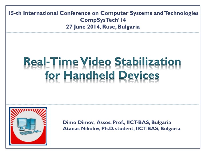
15-th International Conference on Computer Systems and Technologies CompSysTech 14 27 June 2014, Ruse, Bulgaria Real-Time Video Stabilization for Handheld Devices Dimo Dimov, Assos. Prof., IICT -BAS, Bulgaria Atanas Nikolov, Ph.D. student, IICT -BAS, Bulgaria

1. Introduction (2) Video stabilization seeks to create a stable version of casually shot video (usually filmed on a handheld device, such as a mobile phone or a portable camcorder) which is typically shaky and undirected, i.e. it suffers from all the disadvantages of a non-stationary camera filming. By contrast, professional cinematographers carefully plan camera motion along smooth simple paths, using a wide variety of sophisticated equipment, such as tripods, cameras mounted on rails, camera dollies, steadicams, etc. Such hardware is impractical for many situations (or expensive for amateurs), so the software video stabilization is a widely-used for improving casual video. 2

1. Introduction In principle, the task of software 2D stabilization (and even 3D stabilization) is considered solved in the cases of an off-line processing, and even in real time, but if using a powerful enough computer and a parallel implementation on the GPU. However, at least for now, the computing power of mobile phones is not enough to achieve acceptable video stabilization and therefore it is relied also on the usage of the inertial sensors (gyroscopes and/or accelerometers) in the phone s hardware. The method proposed here concerns the 2D video stabilization and aims at achieving minimal implementation complexity in a combination with enough precision, so that it can be used as a periodical initializing contrivance for the system of inertial sensors in the mobile phone, finally responsible for the full (possibly 3D) video stabilization in real time. 2

2.1. 2D Video Stabilization: pros (+) and cons (-) In general, the methods for 2D video stabilization are based on the estimation of an optimal linear transformation of the current frame to a reference one (e.g. previous frame) in a given video sequence. The actual stabilization is realized through a transformation, inverse to the calculated one that converts (translates, rotates, scales, etc.) the current frame to achieve an optimal match to the reference one. In case of approximately plain scenes (with an arbitrary camera movement) or cases where the camera shake is strictly rotational (within an arbitrary scene), unwanted jitters can be effectively reduced based on two-dimensional reasoning of the video. Assuming the scene geometry and camera motion do fall into these categories, such 2D stabilization methods are robust, operate on the entire frame and consume minimal computing efforts. ... 4

2.1. 2D Video Stabilization: pros (+) and cons (-) However, most scenes do contain objects at arbitrary depths and in many scenarios, such as hand-held camera shoots, it is actually impossible to avoid any translational component in the camera shake. In these cases, a full-frame matching cannot model the parallax that is induced by a translational shift in viewpoint and this level of scene modelling is insufficient for video stabilization. The second limitation of these 2D motion models is that there is no knowledge of the 3D trajectory of the input camera, making it impossible to simulate an idealized camera path similar to what can be found in professional tracking shots. 5

2.2. 3D Video Stabilization in Brief The first realization of 3D video stabilization for dynamic scenes was described in the paper: Content-Preserving Warps for 3D Video Stabilization (Liu et al. 2009). But, despite achieved high quality of movement smoothness there, its application was practically limited by the need of carrying out a 3D reconstruction of scenes through SFM (Structure from Motion) method. SFM has restrictions towards robustness and generality because some videos simply do not contain sufficient motion information to allow for reconstruction. These restrictions are: (1) Parallax (because of depth of the real scene); (2) Camera zooming; (3) In-camera stabilization (the img sensor instead the lenses); (4) Rolling shutter (of CMOS performances, but not for CCD). (5) Other (lenses, atmospheric blur, in-scene motions, ...) Beyond this restrictions, the processing speed was also a significant problem there, because SFM requires a global nonlinear optimization. Because of the above mentioned problems with 3D video stabilization, a trend has appeared recently toward the usage of 2D approaches, because of their computational efficiency and robustness. 6

2.3. Interesting Methods for 2D Video Stabilization An evidentiary fast (over 100 fps for 1280x960 video) and simple approach for 2D video stabilization (but for translation only) was described in the White Paper of Texas Instruments: Motion Stabilization for Embedded Video Applications (Fitzgerald, 2008). We are interested in this method because it uses the BSC chip from the TMS320DM365 digital media processor based on DaVinci technology of TI. BSC enables an efficient calculation of the integral projections of an image, i.e. vertical and horizontal sums by pixels. More precisely, BSC can uniformly break up the input image into parts e.g. into 9 sub-images (3x3), on which to calculate the respective 18 integral projections (or 'histograms'), i.e. by 2 histograms for each sub-image. Another interesting development of TI (later patented), claiming to be the first one, that jointly treats classical 2D stabilization and stabilization against the rolling shutter effect is: Video Stabilization and Rolling Shutter Distortion Reduction (Hong, 2011): ( sin ) 7

2.3. Interesting Methods for 2D Video Stabilization (2) See, the paper, Eq.1. Because of this, we call their modeling transformation: approximated matrix model . In contrast, we offer graphically clear an accurate vector model of changes between successive frames, which also allows for finding of the elementary geometric transformations translation, rotation, scale, skew, etc. Simple approaches to motion vectors evaluation: - unregular distrubution of characterictic points (SfM) frames regular division on subimages; - directly from MPEG: not very good idea, because of only for basic frames; - via 2D differences for each couple of consecutive frames: - in L2 => (Euclidian distance) => 2D correlation => usage of FFT to speed up - in L1 => (Manhattan): SAD (Sum of Absolute Differences): better but slow - Resp. approximations via horizontal & vertical histograms (sum of intensities): 8

3. Description of Our Method for Video Stabilization 3.1. Evaluation of the Motion Vectors Before considering the Accurate Vector Model (AVM) of our method, we will give a brief description of the basic scheme for determining of the so called motion vectors , similarly to the TI developments, but with our improvements. ? 1 ?V ?V IPV?? ?H ?H ?H ??? (0,1) (0,0) (0,2) ? IPV?? ?V ?size ?wsiz (1,0) (1,1) (1,2) ?wsiz ? 1 IPH?? (2,0) (2,1) (2,2) ? ?size IPH?? 9

3. Description of Our Method for Video Stabilization 3.1. Evaluation of the Motion Vectors (2) Our improvement consists of the following: instead of the conventional IPH?? use in the above calculation the normalized projections, IPH their average, moreover - the average is a floating one. For example, along horizontals we have: ? and IPV?? ?, i.e. centralized by ?, we ?? ?? ? and IPV ?wsiz/2 1 ? ?, = IPH?? ? , IPH ? = ? + ? IPH ?? ?? ?? , ? ? IPH IPH?? ?wsiz ?= ?wsiz/2 as well as by analogy along verticals. (?)) ? ,???? Similarly, as in the papers of TI, the respective 9 motion vectors for the k-th frame, are estimated as a minimum by the SAD approach: ? ??= (???? ?wsiz/2 ? = argmin ? ; SADH?? ? = ? ? + IPH?? , ?H< < ?H; ? 1 ? SADH?? IPH?? ???? ?= ?wsiz/2 ?wsiz/2 (?)= argmin ? ; SADV?? ? = ? ? + IPV?? , ?V< < ?V . ? 1 ? SADV?? IPV?? ???? ?= ?wsiz/2 10

3. Description of Our Method for Video Stabilization 3.2. Description of the Accurate Vector Model (AVM) (0,0) (0,1) (0,2) ? 00 ? 01 ? 02 ? 00 + ? 00 ? 01 ? 02 ? 02 ? 01 The considering only a translation and a rotation two (possibly con- secutive) frames of a video. basic AVM ? (1,1) (1,0) (1,2) ? 10 ? 12 between ? 11 ? 11 ? 10 ? 10 ? 12 ? ? 12 ? ?wsiz ?wsiz (2,1) (2,0) (2,2) ? 20 ? 21 ? 22 diag ? 21 ? 20 ? 20 ? 22 ? 21 ? 22 ? In the proposed here basic AVM, each motion vector ? ??, measured by SAD, between two Fig.2: The basic AVM considering only a translation and a rotation between two (possibly consecutive) frames of a video. frames, is decomposed into a sum of two vectors: a translation ? ?? and a rotation vector ? ??, i.e. ? ??= ? ??+ ? ??. 11

3. Description of Our Method for Video Stabilization 3.2. Description of the Accurate Vector Model (AVM) (2) Thereby, we form 9 vector equations, one for each pair of centres (??? (? = 0,1,2), (? = 0,1,2) in given two (notnecessarilyconsecutive) frames ? 1 and (?), ? = 1,2, from the video clip. The unknown parameters are: the translation vector ? = (?? , ??), which is one and the same (? ??= ? ) for each pair of centres; and the referencerotation vector? = ??,??, which is chosen to be ? = ? 12= ??12,??12, and by which the remaining rotation vectors ? ?? are expressed (for one and the same angle ?). Thus, we compose a system of 18 component equations for the 4 unknowns (??, ??, ??, ??), and we find them by LSM, see Table 1. ? 1), ?, ??? Table 1. LSM equationsof the proposedbasic AVM. 2 LSM on ?? 2 2 2 Centre (j,i) xji yji xji yji LSM on ?? r 2 r 2 r 2 r 2 y y x x = = T t T t 0 0 0 0 (1,1) 11 11 y y y 11 x 11 x x + + = = = = + + = = = = T r t T T r r t t 0 0 (1,2) 12 12 12 y y y y y 12 x 12 x 12 x x x T r t 0 k k 0 (1,0) 10 10 10 y y y y y 10 x t 10 x 10 x x x k k T kr T kr t 0 0 (2,1) 21 21 21 21 21 x y x x y x y y y 21 x T kr t T kr t 0 0 (0,1) 01 01 01 01 01 x y x x y x y y y 01 x + + + + = = = = + + + + = = = = k k k k k k k k T r kr t T kr r t (2,2) 22 22 22 22 22 22 x x y x x y x y y y y y 22 22 x x y T r kr t T kr r t (0,0) 00 00 00 00 00 00 x x y x x y x y y y y 00 00 x x T r kr t T kr r t (0,2) 02 02 02 02 02 02 x x y x x y x y y y y y 02 02 x x x T r kr t T kr r t (2,0) 20 20 20 20 20 20 x x y x x y x y y y y y 20 20 x 12

3. Description of Our Method for Video Stabilization 3.2. Description of the Accurate Vector Model (AVM) (3) Besides the classical matrix approach (as far as the case of LSM is linear), the searched optimal solution for (??, ??, ??, ??), can be calculated by the global minimum of the objective function i j i j , , 2 = = + 2 2 , namely by solving a system of 4 equations ( ) L ji xji yji L L L L by zeroing the respective first partial derivatives , , and (in case of non- y T x T yr xr negativity of the second partial derivatives). Under this more general approach, the following direct solution can be obtained: 1 , 9 , , i j i j ( ) ( k + ( ) ( k + which is more efficient for real time use than the classical matrix approach for linear LSM. 1 = = ; T t T t x xji y xji 9 t + + + + + ) t t t t t k t t t t t t 12 x 10 x 22 00 02 20 21 01 22 00 02 20 x x x x y y y y y y = , r x 2 6 6 + + + + ) t t t t t t k t t t t t t 12 10 22 00 02 20 6 21 01 22 00 02 20 y y y y y y x x x x x x = = , ; r 2 arctg ( / ) x r r y y 2 6 13

3. Description of Our Method for Video Stabilization 3.3. Improvements of the Proposed Basic Algorithm To increase the accuracy of the found solution we apply LSM second time, but on a smaller number of equations for the searched unknowns (??, ??, ??, ??). For this purpose, it is enough to introduce new parameters ???, (? = 0,1,2), ? = 0,1,2, as follows: ???= 0, if the equation (?,?) will be eliminated, otherwise ???= 1. Thus, for the second LSM, we get a modified system of 18 equations, see Table 2. Table 2. LSM equationsof the extended AVM. 2 2 2 2 2 2 2 2 Centre (j,i) yji r xji r yji r xji r e e e e LSM on ?? LSM on ?? xji xji yji yji x y y x ( ( T ( T ( T ( T ) ) ) ( ( ( T ( T ) ) ) = = T t e (1,1) T t e 0 0 0 0 11 y 11 y 11 y y 11 x 11 x 11 x x + + = = = = y e y e + = r r kr kr t t e e ) ) T r t e x e (1,2) (1,0) (2,1) (0,1) (2,2) ( (0,0) ( (0,2) ( (2,0) ( 0 0 0 0 12 y 12 y 12 y 12 12 y y y 12 x 12 x 12 x 12 12 x x x = = = T r t e ) x e 10 y t t 10 y 10 y e e ) 22 10 0 0 10 y y y 10 x t t 10 x 10 x e ) e 10 0 0 10 x x x ( + ke ke ke kr kr 21 21 21 21 21 21 21 21 x y x x x y x y y y y y 21 21 x x ke 01 01 01 ) e ) e ) e ) e 01 01 01 01 y 01 x y x x x y x y y y y 01 01 x x ( ( ( ( t t t + + + = = = = + + + + = = = = ke ke ke ke T T T T r r r r kr kr kr + kr t t t t T T kr kr kr kr + r r r r e e e ) e y e x e ke 22 22 22 22 22 22 22 22 22 x x y x x x y x y y y y y y y 22 22 22 22 x x x ) ) y e x e ke 00 00 00 00 00 00 00 00 00 00 x x y x x x y x y y y y y y y 00 00 00 00 x x x T T y e y e x e ke 02 02 y 02 02 x x 02 02 02 02 02 02 02 02 x x y x x x y x y y y y y y 02 02 x x e t ke 20 20 y 20 20 x x 20 20 20 20 20 20 20 20 x x y x x x y x y y y y y y 20 20 x 14

3. Description of Our Method for Video Stabilization 3.3. Improvements of the Proposed Basic Algorithm (2) In the proposed method, we assume a Gaussian distribution of the error offsets, , (? = 0,1,2), (? = 0,1,2), obtained at the first LSM pass. Thus, we evaluate 18 coefficients, of the type ???? and ???? , as follows: ????=0, if ???> ? 1, if ??? ? deviations ? ?,? and ? mean values, ? and ?; and is an expertcoefficient, 1 < < 3. The primary idea is to eliminate the equations, giving relatively large deviations at the first LSM pass. and xji yji , and similarly for???? ,where ? and ? arethe mean square 2= 2= 1 9( ??? x)2 1 9( ??? ?)2 ?,? , towards corresponding Table 2. LSM equationsof the extended AVM. 2 2 2 2 2 2 2 2 Centre (j,i) yji r xji r yji r xji r e e e e LSM on ?? LSM on ?? xji xji yji yji x y y x ( ( T ( T ( T ( T ) ) ) ( ( ( T ( T ) ) ) = = T t e (1,1) T t e 0 0 0 0 11 y 11 y 11 y y 11 x 11 x 11 x x + + = = = = y e y e + = r r kr kr t t e e ) ) T r t e x e (1,2) (1,0) (2,1) (0,1) (2,2) ( (0,0) ( (0,2) ( (2,0) ( 0 0 0 0 12 y 12 y 12 y 12 12 y y y 12 x 12 x 12 x 12 12 x x x = = = T r t e ) x e 10 y t t 10 y 10 y e e ) 22 10 0 0 10 y y y 10 x t t 10 x 10 x e ) e 10 0 0 10 x x x ( + ke ke ke kr kr 21 21 21 21 21 21 21 21 x y x x x y x y y y y y 21 21 x x ke 01 01 01 ) e ) e ) e ) e 01 01 01 01 y 01 x y x x x y x y y y y 01 01 x x ( ( ( ( t t t + + + = = = = + + + + = = = = ke ke ke ke T T T T r r r r kr kr kr + kr t t t t T T kr kr kr kr + r r r r e e e ) e y e x e ke 22 22 22 22 22 22 22 22 22 x x y x x x y x y y y y y y y 22 22 22 22 x x x ) ) y e x e ke 00 00 00 00 00 00 00 00 00 00 x x y x x x y x y y y y y y y 00 00 00 00 x x x T T y e y e x e ke 02 02 y 02 02 x x 02 02 02 02 02 02 02 02 x x y x x x y x y y y y y y 02 02 x 15 x e t ke 20 20 y 20 20 x x 20 20 20 20 20 20 20 20 x x y x x x y x y y y y y y 20 20 x

4. Experimental Analysis For a quantitative analysis of our algorithms quality, we use Interframe Transformation Fidelity (ITF) metrics: ? 1 1 , ? 1PSNR ? , ? 1 ?=1 ITF = where PSNR is a peak signal-to-noise ratio between twoconsecutive frames (? 1) and (?), and ? is the number of frames in the video clip. The PSNR measures the degree of similarity between two images, which makes it suitable for the evaluation of the proximity between frames: PSNR ? , ? 1= 10log10MSE ? , ? 1, where ?size 1 ?size 1 1 , MSE ? , ? 1= diff ?? ?,? ,?? 1 ?,? 1 + ?size?size ?=0 ?=0 where ?? ?,? is the value of pixel ?,? in ? -th frame, and diff ?,? =1, if ? ? > ? , 0 ?|? 255, 0, otherwise where ? is a threshold, ? 255. We define experimentally the threshold value ? = 32, so that it is suitable for our test videos. The aim is ITF to give sufficientlydifferent results between an original and stabilized video and between videos, stabilized by the different methods compared here. 16

4. Experimental Analysis (2) Experiments have been conducted on 5 video clips of frame size (640x480), with a different degree of jittering, assessed on a scale from 1 (for low) to 5 (for strong), see Fig. 3. The respective ITF values for the quality of the experimented approaches by our method for stabilization, in these test videos, are shown in Table 3. The experiments are ++ and/or Matlab written in Windows 7, and are carried out on an Intel Q9550 CPU 2.83 GHz, RAM 12GB, HDD 7200 rpm. 1 2 3 4 5 Fig.3: Tested video clips ordered increasingly by their degree of shaking (a frame is only shown per clip). Table 3. ITF measures for 5 video-clips: the originals and their stabilization by 6 approaches. method video 1 11.85 16.57 17.45 2 11.09 14.36 16.06 3 10.01 14.02 14.79 4 9.61 13.05 13.66 5 9.40 12.58 13.07 1 2 3 4 5 6 7 original 3x3/noAVG/I 3x3/AVG/I 3x3/noAVG/II 3x3/AVG/II 9x9/AVG/II FAST 17.68 16.01 14.84 13.85 13.17 17.99 16.43 15.30 14.03 13.29 17.99 16.29 15.51 14.31 13.32 18.09 16.37 15.70 14.32 13.40 AVM [ms] Totals [ms] [fps] - 6 5 5 7 110 9.09 37 141 7.09 ( 52 ) 156 6.41 33 30 111 9.02 109 9.18 111 9.00 17 1(original): the ITF values of the original (unstabilized) videos are given in the column; 2(3x3/noAVG/I) uses 3x3 division schema, without any IP normalization and applies LSM only once; 3 (3x3/AVG/I): the same as above, but with normalization of the integral projections (IP); 4 (3x3/noAVG/II): uses 3x3 division, without normalizing of IP, but applies LSM for second time (LSM-II); 5 (3x3/AVG/II): the same of above, and an IP normalization applied; 6(9x9/AVG/II): uses 9x9 division schema, an IP normalization and LSM-II as well; 7(FAST): the FAST method [16] (implemented in Computer Vision Toolbox of Matlab) is used to find corresponding feature points in two frames. To improve the accuracy of the found matches, we also use the outside Matlab code, implementing the RANSAC algorithm [6, 11].

4. Experimental Analysis (3) Table 3. ITF measures for 5 video-clips: the originals and their stabilization by 6 approaches. method video 1 11.85 16.57 17.45 2 11.09 14.36 16.06 3 10.01 14.02 14.79 4 9.61 13.05 13.66 5 9.40 12.58 13.07 1 2 3 4 5 6 7 original 3x3/noAVG/I 3x3/AVG/I 3x3/noAVG/II 3x3/AVG/II 9x9/AVG/II FAST 17.68 16.01 14.84 13.85 13.17 17.99 16.43 15.30 14.03 13.29 17.99 16.29 15.51 14.31 13.32 18.09 16.37 15.70 14.32 13.40 AVM [ms] Totals [ms] [fps] - 6 5 5 7 110 9.09 37 141 7.09 ( 52 ) 156 6.41 33 30 111 9.02 109 9.18 111 9.00 For the C++ version, the pure durations of our method are given on row 6 of Table 3. Subtracting them from the totals (see row 7), the rest obviously dominate and can be shared out on average as follows: for read 15 ms, for image reverse transform 75 ms, for save 10 ms, and for extra operations 5 ms. Thus, the achieved maximal speed (in fps) is 7 9 fps. We assume these outside operations can be executed quite more efficiently on the special hardware of a handheld device; e.g. 3 times faster will be enough to achieve the conventional speed of 30 fps. 18 1(original): the ITF values of the original (unstabilized) videos are given in the column; 2(3x3/noAVG/I) uses 3x3 division schema, without any IP normalization and applies LSM only once; 3 (3x3/AVG/I): the same as above, but with normalization of the integral projections (IP); 4 (3x3/noAVG/II): uses 3x3 division, without normalizing of IP, but applies LSM for second time (LSM-II); 5 (3x3/AVG/II): the same of above, and an IP normalization applied; 6(9x9/AVG/II): uses 9x9 division schema, an IP normalization and LSM-II as well; 7(FAST): the FAST method [16] (implemented in Computer Vision Toolbox of Matlab) is used to find corresponding feature points in two frames. To improve the accuracy of the found matches, we also use the outside Matlab code, implementing the RANSAC algorithm [6, 11].

4. Experimental Analysis (4) The following conclusions can also be drawn based on the experiment results: ITF evaluations correspond to the degree of camera shaking, and we believe it is adequate to our visual classification (i.e., the higher ITF the better stabilized video); The worst ITF results are obtained by (3x3/noAVG/I)-approach, i.e. when neither IP (integral projections) normalization nor the second LSM pass (LSM-II) is used; The (3x3/noAVG/II)-stabilization is almost as unacceptable as the (3x3/AVG/I)-one, but according to the estimated ITF, it follows that LSM-II has a higher impact on the output result quality, rather than the IP normalization; The quality of results (visually and by ITF) is significantly increased at (3x3/AVG/II), i.e. at acombination of both, the IP normalization and the LSM-II; Usage of more detailed division scheme causes (compare (9x9/AVG/II) and (3x3/AVG/II)) better stabilization of/on videos of low quality (less ITF) than of/on better quality videos (high ITF); The most pleasant results, as expected, have been obtained by the (FAST) method, and it is well visible in/on videos of bad quality; It is observed that at 9x9 division schema, the result is the closest to this of (FAST) method, i.e. the approach of more detailed uniform division could reach the results with feature points like (FAST), which determines the trend of our future work. 19

Live demo is avaiable

5. Conclusion An innovative, efficient and robust method for 2D video stabilization is presented here, which is designed for real-time working on portable devices. The BSC (Boundary Signal Computation) chip of TI (Texas Instruments) is emulated herein for searching of correlations between the 1D integral projections, horizontal and vertical ones by the SAD (Sums of Absolute Differences) approach. The proposed method is based on an accurate vector model of the motion, allowing interpretations of increasing complexity for the transformations among frames (e.g. considering of scaling, skew). The method is intended as an initializing tool for the system of inertial sensors of a mobile device, finally responsible for the actual video stabilization. 21

References [1] Batur, A. U., B. Flinchbaugh, Video Stabilization with Optimized Motion Estimation Resolution, IEEE International Conference on Image Processing, 2006, pp. 465-468. Fitzgerald, J. A., Translational Motion Stabilization for Embedded Video Applications, White Paper SPRAAX8, 2008, Texas Instruments. Goldstein, A., and R. Fattal, Video stabilization using epipolar geometry, ACM Transactions on Graphics, 2012, Vol. 31 (5), pp. 126:1-126:10. Grundmann, M., V. Kwatra, and I. Essa, Auto-directed video stabilization with robust L1 optimal camera paths, In 2011 Conference on Computer Vision and Pattern Recognition (CVPR), 2011, pp. 225-232. Hanning, G., N. Forslow, P.-E. Forssen, E. Ringaby, D. Tornqvist, J. Callmer, Stabilizing cell phone video using inertial measurement sensors, 2011 IEEE International Conference on Computer Vision Workshops, 2011, pp. 1-8. Hartley, R. I., and A. Zisserman, Multiple View Geometry in Computer Vision, Cambridge University Press, 2003. Hong, W., D. Wei, A.U. Batur, Video Stabilization and Rolling Shutter Distortion Reduction, Proc. of 17th IEEE International Conf. on Image Processing (ICIP), 2010, pp. 3501-3504. Hong, W., D. Wei, A.U. Batur, Video Stabilization and Reduction of Rolling Shutter Distortion, US Patent Application Publication, No.: US 2011/0176014 A1, Date: Jul. 21, 2011. Jia, C., and B. L. Evans, Probabilistic 3-D Motion Estimation for Rolling Shutter Video Rectification from Visual and Inertial Measurements, Proc. IEEE Multimedia Signal Processing Workshop, 2012,The University of Texas at Austin. Karpenko, A., D. Jacobs, J. Baek, and M. Levoy, Digital video stabilization and rolling shutter correction using gyroscopes, Stanford University Computer Science Tech Report 2011-03. Kovesi, P., MATLAB and Octave Functions for Computer Vision and Image Processing, http://www.csse.uwa.edu.au/~pk/research/matlabfns/ Liu, F., M. Gleicher, H. Jin, and A. Agarwala, Content-preserving warps for 3D video stabilization, ACM Transactions on Graphics, 2009,Vol. 28 (3), pp. 44:1-44:9. Liu, F., M. Gleicher, J. Wang, H. Jin, and A. Agarwala, Subspace video stabilization, ACM Transactions on Graphics, 2011,Vol. 30 (1), pp. 4:1-4:10. Liu S., L. Yuan, P. Tan, and J. Sun, Bundled camera paths for video stabilization, ACM Transactions on Graphics, 2013, Vol. 32 (4), Article No. 78. Marcenaro, L., G. Vernazza, C. S. Regazzoni, Image stabilization algorithms for video-surveillance applications, IEEE Int. Conf. on Image Processing, 2001, Vol. 1, pp. 349-352. Rosten, E., R. Porter, and T. Drummond, FASTER and better: A machine learning approach to corner detection, IEEE Transaction on PAMI, 2010, Vol. 32, pp. 105-119. TMS320DM365 Video Stabilization Algorithm Datasheet, January 2010, Texas Instruments. Wang, Y.-S., F. Liu, P.-S. Hsu, and T.-Y. Lee, Spatially and Temporally Optimized Video Stabilization, IEEE Transaction on VCG, 2013, Vol. 19 (8), pp. 1354-1361. [2] [3] [4] [5] [6] [7] [8] [9] [10] [11] [12] [13] [14] [15] [16] [17] [18] 22

THANK YOU