Recent Trends in Time-Frequency Analysis

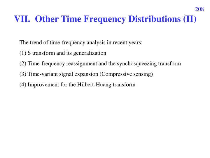
208 VII. Other Time Frequency Distributions (II) The trend of time-frequency analysis in recent years: (1) S transform and its generalization (2) Time-frequency reassignment and the synchosqueezing transform (3) Time-variant signal expansion (Compressive sensing) (4) Improvement for the Hilbert-Huang transform

209 VII-A S Transform (Modification from the Gabor transform) ( ) ( ) ( ) 2 = 2 ( , ) exp exp 2 x S t f f x t f j f d closely related to the wavelet transform advantages and disadvantages [Ref] R. G. Stockwell, L. Mansinha, and R. P. Lowe, Localization of the complex spectrum: the S transform, IEEE Trans. Signal Processing, vol. 44, no. 4, pp. 998 1001, Apr. 1996.

210 S transform Gabor transform Gaussian window f ( ) = 2 ( ) exp w t t = 2 2 exp w t f t f worse time resolution, better frequency resolution better time resolution, worse frequency resolution The result of the S transform (compared with page 94) 3 6 2 4 f-axis 1 2 0 0 -1 -2 -2 -4 -6 -3 0 5 10 15 20 25 t-axis

211 General form ( ) s f ( ) ( ) ( ) f ( ) 2 = 2 ( , ) exp exp 2 x S t f x t s j f d s(f) increases with f C. R. Pinnegar and L. Mansinha, The S-transform with windows of arbitrary and varying shape, Geophysics, vol. 68, pp. 381-385, 2003.

212 Fast algorithm of the S transform When f is fixed, the S transform can be expressed as a convolution form: ( ) s f ( ) ( ) ( ) f ( ) 2 = 2 ( , ) exp exp 2 x S t f x t s j f d ( ) s f ( ) x t ( ) ( ) f = 2 2 t s ( , ) S t f exp 2 exp j ft x convolution along t axis (for every fixed f) = ( ) ( ( ) ( ) ) g t h t g h t d Remember: Q: Can we use the FFT-based method on page 119 to implement the S transform?

213 VII-B Generalized Spectrogram [Ref] P. Boggiatto, G. De Donno, and A. Oliaro, Two window spectrogram and their integrals," Advances and Applications, vol. 205, pp. 251-268, 2009. ( ) ( ) ( ) = , , , SP t f G t f G t f Generalized spectrogram: , , , , x w w x w x w 1 2 1 2 ( ) ( ) ( ) x = 2 j f , G t f w t e d , 1 x w 1 ( ) ( ) ( ) x = 2 j f , G t f w t e d , 2 x w 2 Original spectrogram: w1(t) = w2(t) To achieve better clarity, w1(t) can be chosen as a wider window, w2(t) can be chosen as a narrower window.

214 x(t) = cos(2 t) when t < 10, x(t) = cos(6 t) when 10 t < 20, x(t) = cos(4 t) when t 20 (a) Gabor, sigma = 0.1 5 f-axis 0 -5 0 5 10 15 20 25 30 t-axis (b) Gabor, sigmal = 1.6 5 f-axis 0 -5 0 5 10 15 20 25 30 t-axis

215 x(t) = cos(2 t) when t < 10, x(t) = cos(6 t) when 10 t < 20, x(t) = cos(4 t) when t 20 (c) Generalized spectrogram 5 f-axis 0 -5 0 5 10 15 20 25 30 t-axis (d) Gabor, sigmal = 0.4 5 f-axis 0 -5 0 5 10 15 20 25 30 t-axis

216 ( ) ( ) ( ) = , , , SP t f G t f G t f Generalized spectrogram: , , , , x w w x w x w 1 2 1 2 Further Generalization for the spectrogram: ( ) ( ) ( ) = , , , SP t f G t f G t f , , , , x w w x w x w 1 2 1 2 or ( ) ( ) ( ) = , , , SP t f G t f G t f , , , , x w w x w x w 1 2 1 2

217 VII-C Reassignment Method After computing the time-frequency distribution, we can use the following way to make the energy even more concentrated. (1) First, estimate the offset. ? ? ?,? ? ? ?,? ???? ? ?,? = ? ?,? ? ? ?,? ???? (t, f ) ? ? ?,? ? ? ?,? ???? ? ?,? = ( ) ( ) ( ) f t f , t t f , , ? ?,? ? ? ?,? ???? X(t, f): time-frequency analysis (STFT, WDF ) of x(t), (u, v) = 1 when |u|, |v| < B (u, v) = 0 otherwise ? ?,? ? ( ) ( ) ( ) f t f , t t f , , (2) Then, shift the time frequency distribution at (t, f ) to

218 ( ) ( ) ( ) f t f , t t f , , (2) Then, shift the time frequency distribution at (t, f ) to ( ) ( ) ( ) ( ) ( ) ( ) f t f = t t f , , , , X t f X t f t f dt df 1 1 1 1 1 1 1 1 References [1] F. Auger and P. Flandrin, Improving the readability of time-frequency and time-scale representations by the reassignment method, IEEE Trans. Signal Processing, vol. 43, issue 5, pp. 1068-1089, May 1995. [2] F. Auger, P. Flandrin, Y.T. Lin, S. McLaughlin, S. Meignen, T. Oberlin, and H.T. Wu, Time-frequency reassignment overview, IEEE Signal Processing Magazine, vol. 30, issue 6, pp. 32-41, 2013. and synchrosqueezing: An PS: 2017

219 VII-D Basis Expansion Time-Frequency Analysis M ( ) x t exp( 2 ) a j f t Fourier series: m(t) = exp(j2 fmt), m m = 1 m fm= m/T ( ) ( ) m ( ) ( ) m , x t t 1 T T ( ) x t m = = f t dt exp( 2 ) a j m m , t t 0 Time-Frequency Analysis signal M ( ) x t ( ) t a m m = 1 m M 2 M ( ) x t ( ) t approximation error = a dt m m = 1 m m(t) basis frequency

220 (1) Three Parameter Atoms ( ) x t ( ) t a , , , , t f t f 0 0 0 0 2 1/4 ( ) 2 t t = ( ) t exp( 2 )exp( ) 0 j f t , , 0 t f 1/2 2 0 0 3 parameters: t0controls the central time f0controls the frequency controls the scaling factor [Ref] S. G. Mallat and Z. Zhang, Matching pursuits with time-frequency dictionaries, IEEE Trans. Signal Processing, vol. 41, no. 12, pp. 3397-3415, Dec. 1993. ,( ) t a Since are not orthogonal, should be determined by a matching pursuit process. , , , t f t f 0 0 0 0

221 (2) Four Parameter Atoms (Chirplet) ( ) x t ( ) t a , , , , , , t f t f 0 0 0 0 2 1/4 ( ) 2 t t = + 2 ( ) t exp( 2 ( ) ) 0 j f t t 2 , , 0 t f 1/2 2 0 0 4 parameters: t0controls the central time f0controls the initial frequency controls the scaling factor controls the chirp rate [Ref] A. Bultan, A four-parameter atomic decomposition of chirplets, IEEE Trans. Signal Processing, vol. 47, no. 3, pp. 731 745, Mar. 1999. [Ref] C. Capus, and K. Brown. "Short-time fractional Fourier methods for the time-frequency representation of chirp signals," J. Acoust. Soc. Am. vol. 113, issue 6, pp. 3253-3263, 2003.

222 (a) STFT of a Fourier basis 5 f-axis 0 -5 0 2 4 6 8 10 12 t-axis (b) STFT of a 3-parameter atom 5 f-axis 0 -5 0 2 4 6 8 10 12 t-axis (4-parameter atom) (c) STFT of a chirplet 5 f-axis 0 -5 0 2 4 6 8 10 12 t-axis

223 (3) Prolate Spheroidal Wave Function (PSWF) ( ) x t ( ) ( ) exp 2 , , , , n T a t t j f t , , n T 0 0 t f 0 0 , , , , n T t f 0 0 where is the prolate spheroidal wave function [Ref] D. Slepian and H. O. Pollak, Prolate spheroidal wave functions, Fourier analysis and uncertainty-I, Bell Syst. Tech. J., vol. 40, pp. 43-63, 1961.

224 Concept of the prolate spheroidal wave function (PSWF): ( ) ( ) ( ) f t x t dt = FT: , x, f ( , ). exp 2 X f j energy preservation property (Parseval s property) 2 2 = ( ) ( ) x t X f df dt finite Fourier transform (fi-FT): ( ) exp fi T T ( ) ( ) f t x t dt = 2 X f j space interval: t [ T, T], frequency interval: f [ , ] 2 ( ) f X df fi = 0 energy preservation ratio 1 T 2 ( ) x t dt T 2 ( ) f X df ( ) t fi can maximize The PWSF 0, , T T 2 ( ) x t dt T

225 2 ( ) f X df ( ) t fi can maximize The PWSF 0, , T T 2 ( ) x t dt T 2 ( ) f X df ( ) t fi can maximize 1, , T T 2 ( ) x t dt T 2 ( ) f X df ( ) t fi can maximize 2, , T T 2 ( ) x t dt T and so on.

226 Prolate spheroidal wave functions (PSWFs) are the continuous functions that satisfy: ( ) ( ) , , , 1 , F T 1 , 1 1 ( t t T ( ) 1 t = K t t t d t , , n T , , n T n T , sin 2 . ( t ) t where ( ) = , K t t F ) PSWFs are orthonormal and can be sorted according to the values of n,T, s: ( ) ( ) , , , , m T n T T T = t t dt , m n 1 > 0,T, > 1,T, > 2,T, > . > 0. (All of n,T, s are real)

227 Compressive Sensing and Matching Pursuit Different from orthogonal basis expansion, which applies a complete and orthogonal basis set, compressive sensing is to use an over-complete and non-orthogonal basis set to expand a signal. Example: Fourier series expansion is an orthogonal basis expansion method: M ( ) x t exp( 2 ) a j f t m m = 1 m f t dt = if fm fn exp( 2 )exp( 2 ) 0 j f t j m n Three-parameter atom expansion, Four-parameter atom (chirplet) expansion, and PSWF expansion are over-complete and non-orthogonal basis expansion methods. ( ) 0 0 , , t f x t a ( ) t , , t f 0 0

228 6 5 4 3 2 1 0 -1 -2 -3 -4 0 5 10 15 For example, in the above figure, the blue line is the original signal When using three-parameter atoms, the expansion result is the red line ( ) 3 2.5 x t e e = + Only 3 terms are used and the normalized root square error is 0.39% 2 2 2 0.2 ( 0.4 ( + 0.4 ( + 5) 8) 2 8) 2 t t j t t j t 2.5 e When using Fourier series, if 31 terms are used, the expansion result is the green line and the normalized root square error is 3.22%

229 The problems that compressive sensing deals with: Suppose that b0(t), b1(t), b2(t), b3(t) .. form an over-complete and non-orthogonal basis set. (Problem 1) We want to minimize ||c||0 (|| ||0 L0norm ||c||0 cm 0 such that Sparse: smaller L0 norm = ( ) x t ( ) t m m c b m (Problem 2) We want to minimize ||c||0such that 2 ( ) x t ( ) t m m c b dt threshold m (Problem 3) When ||c||0is fixed to M, we want to minimize 2 M ( ) x t ( ) t m m c b dt = 1 m

230 Question: How do we solve the optimization problems on page 229? Method 1: Matching Pursuit (Greedy Algorithm) atoms: bm(t), m = 1, 2, 3, . ( ) m b t b (normalized) Input: x(t) ( ) t dt = 1 Initial: n = 0, xr(t) = x(t) m ( ) ( ) t dt x t b is maximal Find m such that r m ( ) x t b ( ) t dt = Set n(t) = bm(t), n m xr(t) = xr(t) - n n(t) No ( ) x t ( ) t n = n+1 m m m Yes For Problem 1: Whether xr(t) = 0 For Problem 2: Whether For Problem 3: Whether n = M ( ) t dt 2 rx threshold

231 Method 2: Basis Pursuit Change the L0norm into the L1norm ||c||1 = |c0| + |c1| + |c2| + (Problem 1) We want to minimize ||c||1such that ( ) x t = ( ) t m m c b m (Problem 2) We want to minimize ||c||1such that 2 ( ) x t ( ) t m m c b dt threshold m (Problem 3) When ||c||1 M, we want to minimize 2 ( ) x t ( ) t m m c b dt m

232 1 N = [ ] = x n [ ] x n Norm (L norm): 0 n x n where K is the number of points such that [ ] 0 (L norm) = K lim 0 (Physical meaning: The number of nonzero points) 1 N = L1 norm: [ ] = x n [ ] x n 1 0 n (Physical meaning: Sum of Amplitudes) = 1 N 2 [ ] = x n [ ] x n L2 norm: 2 0 n (Physical meaning: Distance) (L norm) lim Matching Pursuit: Zero order norm 0 Basis Pursuit: First order norm L1 norm The L norm is convex if 1.

233 [Compressive Sensing ] S. G. Mallat and Z. Zhang. Matching pursuits with time-frequency dictionaries, IEEE Trans. Signal Processing, vol. 41, issue 12, pp. 3397- 3415, 1993. ( matching pursuit) S. S. Chen, D. L. Donoho, and M. A. Saunders, Atomic decomposition by basis pursuit, SIAM Journal on Scientific Computing, vol. 20, issue 1, pp. 33-61, 1998. ( basis pursuit) J. F. Mota, J. M. Xavier, P. M. Aguiar, and M. Puschel, Distributed basis pursuit, IEEE Trans. Signal Processing, vol. 60, issue 4, pp. 1942- 1956, 2011. ( basis pursuit ) D. L. Donoho, Compressed sensing, IEEE Trans. Inf. Theory, vol. 52, issue 4, pp. 1289 1306, 2006. ( compressive sensing ) E. J. Cand s and M. B. Wakin, An introduction to compressive sampling, IEEE Signal Processing Magazine, vol. 25, issue 2, pp. 21-30, 2008. ( compressive sensing tutorial ) S. Foucart and H. Rauhut, A Mathematical Introduction to Compressive Sensing, Birhauser, Basel, 2013. compressive sensing) (

234 E. J. Cand s and M. B. Wakin, An introduction to compressive sampling, IEEE Signal Processing Magazine, vol. 25, issue 2, pp. 21-30, 2008. ( compressive sensing tutorial) S. Kunis and H. Rauhut, Random sampling of sparse trigonometric polynomials, II. Orthogonal matching pursuit versus basis pursuit, Foundations of Computational Mathematics, vol. 8, issue 6, pp. 737-763, 2008. ( orthogonal expansion matching pursuit, basis pursuit ) T. T. Do, L. Gan, N. Nguyen, and T. D. Tran, matching pursuit algorithm for practical compressed sensing," in IEEE Asilomar Conf. Signals, Systems and Computers, pp. 581-587. IEEE, Oct. 2008. ( sparsity matching pursuit ) W. He and T. Qu, "Audio lossless coding/decoding method using basis pursuit algorithm," IEEE Int. Conf. Acoustics, Speech and Signal Processing, pp. 552-555, May 2013. ( basis pursuit ) "Sparsity adaptive