Rectangular Waveguide: Structure, Modes, and Wave Propagation Analysis

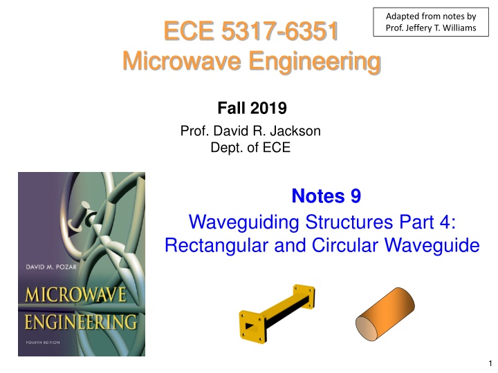
Adapted from notes by Prof. Jeffery T. Williams ECE 5317-6351 Microwave Engineering Fall 2019 Prof. David R. Jackson Dept. of ECE Notes 9 Waveguiding Structures Part 4: Rectangular and Circular Waveguide 1

Rectangular Waveguide One of the earliest waveguides. Still common for high power and low- loss microwave / millimeter-wave applications. It is essentially an electromagnetic pipe with a rectangular cross-section. Single conductor No TEM mode For convenience: a b (the long dimension lies alongx). 2

Rectangular Waveguide (cont.) y Two types of modes: PEC TEz , TMz , , b ( ) 1/2 = 2 2 c k k k z x a z ( ) = = 1 tan k k j 0 c r d = j The cutoff wavenumber kcis real. c We need to solve for kc. = j j c c = j = 2 2 c : f f k k k c c z c = 1 j = 2 c 2 : f f k j k k c c z c = = (1 tan j ) j d (1 tan ) 0 r d 3

TEz Modes For +z propagation: y ( ) ( ) h x y e = jk z , , x y z , H PEC z z z where , , b 2 2 x ( ) + + = 2 c , 0 k h x y z 2 2 x y a z ( ) 1/2 2 2 z k k k c Subject to B.C. s: From previous field table: E x H y j H y = + E k z z = = = 0 0 E z @ 0, y b x z 2 c j k x E y H x = + E k z z H x = y z @ 0, = = x a 2 c 0 0 k E z y 4

TEz Modes (cont.) 2 2 ( ) ( ) + = 2 c , , h x y k h x y (eigenvalue problem) z z 2 2 x y ( ) ( ) ( ) X x Y y = Using separation of variables, let , zh x y 2 2 d X dx d Y dy + = 2 c Y X k XY 2 2 Must be a constant 2 2 1 X dx 1 Y dy d X d Y This is the separation equation . (If we take one term across the equal sign, we have a function of x equal to a function of y.) + = 2 c k 2 2 2 2 1 X dx 1 Y dy d X d Y = = 2 x 2 y k k and 2 2 + = 2 x 2 y 2 c k k k where separation equation 5

TEz Modes (cont.) Hence, ( ) + ( ) + X x Y y ( ) = , ( cos A sin )( cos k x C sin ) h x y k x B k y D k y z x x y y zh y = = 0 @ 0, y b A Boundary Conditions: zh x = @ 0, x a = B 0 n = = = 0 0,1,2,... D k n and A y b m = = = B 0 0,1,2,... B k m and x a 2 2 m x a n y b m n ( ) = = + 2 c , cos cos h x y A k and z mn a b 6

TEz Modes (cont.) Therefore, ( ) 1/2 = 2 2 c k k k m n z ( ) = jk z , , x y z cos cos H A x y e z 1/2 z mn 2 2 a b m n = 2 k a b 2 2 m n From the field table, we obtain the following: = + k c a b j n m n = jk z cos sin E A x y e Note: m n z x mn 2 c k b j a b = = 0,1,2, 0,1,2, m m n = jk z sin cos E A x y e z y mn 2 c k a a b jk m k a jk n k b m n But m = n = 0 is not allowed! = jk z sin cos H A x y e z z x mn 2 c a b m n (non-physical solution) H z A e = = jk z cos sin H A x y e z z y mn 2 c a b jkz ; 0 H 00 7

TEz Modes (cont.) Reason for non-physical solution Start with the vector wave equation: ( ) = 2 0 H k H Vector wave equation: from Maxwell s equations. Take divergence of both sides. ( ) ( ) = 2 0 H k H The divergence of a curl is zero. = 0 H Magnetic Gauss law 8

TEz Modes (cont.) Reason for non-physical solution Revisit how we obtained the vector Helmholtz equation: ( ) H k H = 2 0 Vector wave equation: from Maxwell s equations. ( ) = 2 2 0 H H k H From definition of vector Laplacian H Now use: = 0 H A needed assumption! Magnetic Gauss law + = 2 2 0 H k H Vector Helmholtz equation (what we have solved) 9

TEz Modes (cont.) Reason for non-physical solution Vector wave equation magnetic Gauss law Vector Helmholtz equation magnetic Gauss law The vector Helmholtz equation does not guarantee that the magnetic Gauss law is satisfied. In the mathematical derivation, we need to assume the magnetic Gauss law in order to arrive at the vector Helmholtz equation. All of the modes that we get by solving the Helmholtz equation should be checked to make sure that they do satisfy the magnetic Gauss law. Note: The TE00 mode is the only one that violates the magnetic Gauss law. 10

TEz Modes (cont.) ( ) c = = Lossless case 1/2 ( ) 2 2 m n 1/2 ( ) 2 = = 2 2 mn z mn c k k k k a b ( ) = mn c TEmnmode is at cutoff when k k = mn c k 2 2 1 m a n b = + mn c f 2 Lowest cutoff frequency is for TE10 mode (a > b) 1 = 10 We will revisit this mode later. cf Dominant TE mode (lowest fc) a 2 11

TEz Modes (cont.) At the cutoff frequency of the TE10 mode (lossless waveguide): c c f c = = = = 2 d f d d a 1 d 10 c 2 a so = / 2 a d = f f c 12

TEz Modes (cont.) To have propagation: f f c so 1 f a 2 or 1 1 2 c = = d f d a 2 2 f or d a 2 Example: Air-filled waveguide,f = 10 GHz. We have that a > 3.0 cm / 2 = 1.5 cm. 13

TMz Modes y Recall: PEC ( ) ( ) e x y e = jk z , , x y z , E z z z , , b x where a z 2 2 ( ) ( ) + = 2 c , , e x y k e x y (eigenvalue problem) z z 2 2 x y ( ) 1/2 = 2 2 z k k k c E = = Subject to B.C. s: 0 @ 0, x a z = @ 0, y b Thus, following same procedure as before, we have the following result: 14

TMz Modes (cont.) ( ) + ( ) + X x Y y ( ) = , ( cos A sin )( cos k x C sin ) e x y k x B k y D k y z x x y y = ze = @ 0, 0 y b A Boundary Conditions: = @ 0, x a B n = = = 0 0,1,2,... C k n and A y b m = = = 0 0,1,2,... A k m and B x a 2 2 m n m n = = + 2 c sin sin e B x y k and z mn a b a b 15

TMz Modes (cont.) ( ) 1/2 = 2 2 c k k k Therefore z 1/2 m n 2 2 m n ( ) = jk z = , , x y z sin sin E B x y e 2 k z z mn a b a b 2 2 m n = + k c a b From the field table, we obtain the following: j n m n = = 1,2,3 1,2,3 m n = jk z sin cos c H B x y e z x mn 2 c k b j a b m m n = jk z cos sin c H B x y e z y mn 2 c k a a b Note: If either mornis zero, the field becomes a trivial one in the TMzcase. jk m k a jk n k b m n = jk z cos sin E B x y e z z x mn 2 c a b m n = jk z sin cos E B x y e z z y mn 2 c a b 16

TMz Modes (cont.) Lossless case ( ) c = = (same as for TE modes) 2 2 m n ( ) 2 = = 2 2 mn z mn c k k k k a b 2 2 1 m a n b = + mn c f 2 The lowest cutoff frequency is obtained for the TM11 mode 2 2 1 1 a 1 b = + 11 cf Dominant TM mode (lowest fc) 2 17

Mode Chart y Lossless case ( ) c = = PEC Two cases are considered: , , b b < a / 2 x a z Single mode operation f TE TE TE TE TE TM 10 10 20 01 11 The maximum bandwidth for single-mode operation is 67%. ( b 11 f f ) BW 2 1 / 2 a f 0 b > a / 2 0f =center frequency Single mode operation f 2 2 1 m a n b TE TE TE TE = + mn c f TE TM 10 10 01 20 11 2 11 18

Dominant Mode: TE10 Mode y For this mode we have = = = PEC 10 c 1, 0, m n k a , , b Hence we have x = a jk z 10cos A H x e z z z a 1/2 2 k a = = 10 z 2 k k k = jk z 10sin A H j x e z z z a x a j a = = jk z jk z 10sin A 10sin E E x e E x e z z y y a a E 10 A E 10 10 j a = = = 0 E E H x z y 19

Dominant Mode: TE10 Mode (cont.) The fields can be put in terms of E10: y PEC = jk z 10sin E E x e z y a , , b x 1 = jk z sin H E x e z a 10 x z Z a TE = jk z 10cos E H x e z z j a a 1/2 2 = = 10 z 2 k k k z a = = = = Z 0 E E H TE k x z y z 20

Dispersion Diagram for TE10 Mode Lossless case ( ) c = = 2 = = 2 zk k f f a c = 2 2 k gv = slope 1 10 c (TEMzmode, or Light line ) k = = p v = slope = pv Phase velocity: Velocities are slopes on the dispersion plot. d d = v Group velocity: g 21

Field Plots for TE10 Mode y PEC Top view , , b x a z x E H z a y y b b x a z End view Side view 22

Field Plots for TE10 Mode (cont.) y PEC Top view , , b x a z x sJ H a z y y b b x z a End view Side view Note: One can cut a narrow z-directed slot in the center of the top wall without disturbing the current. 23

Power Flow for TE10 Mode Time-average power flow in the z direction for +z mode: Note: a b 1 2 ( ) + = * zdydx Re P E H 10 a b x ab = 2 sin dydx 0 0 2 a a b 1Re 2 0 0 = * x E H dydx y 0 0 = jk z 10sin E E x e z 1Re 2 ab k y a 2 = 2 z E e z 10 2 1 = jk z sin H E x e z 10 x Z a TE Simplifying, we have = Z TE k z ab k 2 + = 2 z Re P E e 10 10 z 4 At breakdown: Note: For a given maximum electric field level (e.g., the breakdown field), the power is increased by increasing the cross-sectional area (ab). = E E 10 c 24

Dielectric Attenuation for TE10 Mode From Notes 7 we have: f f c = = 2 2 c k j k k z d = 2 2 c Re k k = 2 2 c Im k k d 2 0 2 c k k r r 2 0 tan k r r d d 2 = = = 1 tan ck k k jk k j 0 r r d a 25

Conductor Attenuation for TE10 Mode P+ = P (0) 2 P P (calculated on previous slide) y 0 10 = 0 z = l Recall c 0 sR R b Lossless 2 = (0) s P J d l s 2 x C a z = n s J H on conductor = + + + left right bot top C C C C C 26

Conductor Attenuation for TE10 Mode y sR Side walls = x H = = = left s jk z yH yA e @ 0: x J z 10 z = 0 x b Lossless = = = = jk z right s x H yH yA e @ : x a J z 10 z x x a = a z Hence: = jk z cos H A x e z 10 z a A e = = left sy right sy jk z J J z k a 10 = jk z sin H j A x e z z 10 x a 27

Conductor Attenuation for TE10 Mode (cont.) Top and bottom walls y = y H = bot s @ 0: y J = 0 y sR = = top s y H @ : y b J y b = = top s bot s J J b Lossless (The fields of this mode are independent of y.) x a z Hence: = bot sx jk z cos J A x e z = jk z cos H A x e z 10 a 10 z a k a k a = bot sz jk z sin J j A x e = z jk z sin H j A x e z z z 10 10 x a a 28

Conductor Attenuation for TE10 Mode (cont.) y sR We then have: b Lossless b a R R 2 2 = + left s bot s (0) 2 s s P J dy J dx x l 2 2 0 0 a ) ( z b a 2 2 2 = + + left sy bot sx bot sz R J dy R J J dx s s 0 0 2 2 b a k a 2 = + + cos sin R A dy R A x j A x dx z 10 10 10 s s a a 0 0 2 b a a k a 2 = + + z 2 2 cos sin R A dy x dx x dx 10 s a a 0 0 0 2 2 k a a a 2 = + + z R A b 10 s 2 2 2 29

Attenuation for TE10 Mode (cont.) y Assume f > fc sR (The wavenumber is taken as that of a guide with perfect walls.) zk b Lossless 2 3 a a 2 = + + x (0) P R A b 10 l s 2 2 2 a z = A E ab 10 10 j a 2 = P E 0 10 4 Simplify, using = 10 = ck 2 2 2 c k k a (0) 2 P P = l Final result: c 0 R )( ) = + 2 3 2 2 [np/m] s b a k ( c 3 a b k 30

Attenuation for TE10 Mode (cont.) y sR Final Formulas b Lossless Two alternative forms for the final result: x a z R )( ) = + 2 3 2 2 [np/m] s b a k ( c 3 a b k 2 R b f f 1 2 a b = + 1 [np/m] s c c ( ) 2 1 / f f c 31

Attenuation for TE10 Mode (cont.) Brass X-band air-filled waveguide ( ) 2.6 10 [S/m] 7 : 8 12 [GHz] X band (See the table on the next slide.) a = 2.0 cm (from the Pozar book) 32

Attenuation for TE10 Mode (cont.) Microwave Frequency Bands Letter Designation L band S band C band X band Ku band K band Ka band Q band U band V band E band W band F band D band Frequency range 1 to 2 GHz 2 to 4 GHz 4 to 8 GHz 8 to 12 GHz 12 to 18 GHz 18 to 26.5 GHz 26.5 to 40 GHz 33 to 50 GHz 40 to 60 GHz 50 to 75 GHz 60 to 90 GHz 75 to 110 GHz 90 to 140 GHz 110 to 170 GHz (from Wikipedia) 33

Modes in an X-Band Waveguide = = 2.29cm (0.90in) 1.02cm (0.40in) a b Standard X-band waveguide (WR90) : 8 12 [ X ] band GHz fc [GHz] Mode TE TE TE TE TM TE TE TM 6.55 13.10 14.71 16.10 16.10 19.65 19.69 19.69 1" 10 20 b 0.5" 01 a 11 11 50 mil (0.05 ) thickness 30 21 21 34

Example: X-Band Waveguide a = 2.29cm Determine , ,and g(as appropriate) at 10 GHz and 6 GHz for the TE10 mode in a lossless air-filled X-band waveguide. b = 1.02cm , 0 0 @ 10 GHz 2 2 2 2 10 10 = = 2 8 2.99792458 10 0.0229 a = 158.25[rad/m] 2 2 = = = 0.0397 g 158.25 g = 3.97 [cm] 2 2 2 f = = = = = = Lossless : 2 k f / c f c c 35 d d d d

Example: X-Band Waveguide (cont.) @ 6 GHz 1/2 1/2 2 2 2 9 2 6 10 2.99792458 10 = = 2 zk 8 0.0229 a 2 2 9 2 6 10 2.99792458 10 = j 8 0.0229 = 55.04 [1/m] j = 55.04 [np/m] 478.08[dB/m] = 2 = g Evanescent mode: = 0; gis not defined! 36

Fields of a Guided Wave Fields Equations in Cylindrical Coordinates These are useful for a circular waveguide. E H j = c H k z z z 2 c k These equations give the transverse field components in terms of the longitudinal components, Ezand Hz. E k H j = H z z z c 2 c k y ( ) = jk z F z e z E H j = + E k z z = 2 2 k z 2 c k c = 2 2 z k k k c k E H j = + E z z z 2 c k 37

Circular Waveguide TMz mode: ) , = a , , ( ( ) 2 2 c , e k e z z (eigenvalue problem) PEC = 2 z 2 2 c z k k k This means any combination of these two functions. The solution in cylindrical coordinates is: ( ( ) ) J k Y k sin( cos( ) ) n n ( ) n c = , e z n c Note: The value n must be an integer to have unique fields. 38

References for Bessel Functions = = ( ) ( ) J x Y x n Bessel function of the first kind of order Bessel function of the second kind of order n n n References: M. R. Spiegel, Schaum s Outline Mathematical Handbook, McGraw-Hill, 1968. M. Abramowitz and I. E. Stegun, Handbook of Mathematical Functions with Formulas, Graphs, and Mathematical Tables, National Bureau of Standards, Government Printing Office, Tenth Printing, 1972. N. N. Lebedev, Special Functions & Their Applications, Dover Publications, New York, 1972. 39

Plot of Bessel Functions 1 1 0.8 (0) n J is finite n =0 0.6 n =1 0.4 Jn (x) n =2 J0 x ( ) J1 x ( ) 0.2 Jn 2 x ( ) 0 0.2 0.4 0.403 0.6 0 1 2 3 4 5 6 7 8 9 10 0 xx 10 1 n 2 n = n ( ) ~ J x 0,1,2,...., 0 x n x ( ) ~ J x cos , x x n n 2 ! n 2 4 x 40

Plot of Bessel Functions (cont.) 1 0.521 n =0 0 n =1 1 n =2 2 (0) n Y is infinite Yn (x) Y0 x ( ) Y1 x ( ) 3 Yn 2 x ( ) 4 5 6 6.206 7 0 1 2 3 4 5 6 7 8 9 10 x 0 x 10 + 2 x = ( ) ~ Y x ln , 0.5772156, 0 x 0 2 2 n ( ) ~ Y x sin , x x n 1 2 x n 2 4 x = ( ) ~ ( 1)! , 1,2,3,....., 0 n Y x n n x 41

Circular Waveguide (cont.) n Choose (somewhat arbitrarily) cos( ) ( ( ) ) J k Y k ( ) n c = , cos( ) e n z n c The field should be finite on the z axis. Y k ( ) is not allowed n c ( ) = , cos( ) ( ) e n J k Hence, we have z n c ( ) = jk z , , cos( ) ( ) E z n J k e z z n c 42

Circular Waveguide (cont.) ( ) , , = J k a = 0 z E a z ( ) 0 Hence B.C. s: n c Sketch for a typical value of n(n 0). ( ) n J x Note: Pozar uses the notation pmn. nx 3 x nx nx 1 2 x = np a = k a x k c np c = Note: The value xn0 = 0 is not included since this would yield a trivial solution: ( ) 0 (This is true unless n = 0, in which case we cannot have p = 0.) = 0 J x J 0 n n n a 43

Circular Waveguide (cont.) TMnp mode: ( ) = = jk z , , cos( ) 0,1,2 E z n J x e n z z n np a 2 x np a = = 2 1,2,3,......... k k p z 44

Cutoff Frequency: TMz = 2 z 2 2 c k k k Assume k is real here. x np a zk = = = 0 k k At f = fc : c x np a = TM c 2 f c c = TM d f x c c np d 2 a r 45

Cutoff Frequency: TMz (cont.) xnp values 0 1 2 3 4 5 p \ n 1 2.405 3.832 5.136 6.380 7.588 8.771 2 5.520 7.016 8.417 9.761 11.065 12.339 3 8.654 10.173 11.620 13.015 14.372 4 11.792 13.324 14.796 TM01, TM11, TM21, TM02, .. 46

TEz Modes Proceeding as before, we now have that ( ) = jk z , , cos( ) ( ) H z n J k e z z n c ( ) , , = 0 E a z Set ( ) = 0 H = a H 1 H = (From Ampere s law) E z j z c H = 0 z = a n = The prime denotes derivative with respect to the argument. ( ) 0 J k a Hence c 47

TEz Modes (cont.) n = ( ) 0 J k a c n J x ( ) Sketch for a typical value of n (n 1). nx 3 x nx nx 1 2 np = k a x c x np a = = 1,2,3,..... k p We don t need to consider p = 0; this is explained on the next slide. c 48

TEz Modes (cont.) ( ) np = = jk z , , cos( ) 1,2, H z n J x e p z z n a x = 0 Note: If p = 0, then np We then have, for p = 0: ( ) 0 np = = 0 J x J (trivial solution) n 0 n n a ( ) np = = n = 00 1 J x J 0 0 a = = = jk z jk z jkz ze ze H e H H (nonphysical solution) (violates the magnetic Gauss law) z z z The TE00 mode is not physical. 49

Circular Waveguide (cont.) TEnp mode: ( ) np = = jk z , , cos( ) 0,1,2 H z n J x e n z z n a 2 x np a = = 2 1,2,3,......... k k p z 50