Reducing Coupled Differential Equations for Suspension System Modeling

Modeling a suspension system of a bus involves deriving differential equations to represent the system's behavior. This task requires an understanding of vibrations theory and mathematical techniques. The equations govern the behavior of the suspension mass, spring constants, damping constants, and displacements. By reducing the coupled equations, a simplified model can be created to analyze and predict the system's response.

Download Presentation

Please find below an Image/Link to download the presentation.
The content on the website is provided AS IS for your information and personal use only. It may not be sold, licensed, or shared on other websites without obtaining consent from the author.If you encounter any issues during the download, it is possible that the publisher has removed the file from their server.
You are allowed to download the files provided on this website for personal or commercial use, subject to the condition that they are used lawfully. All files are the property of their respective owners.
The content on the website is provided AS IS for your information and personal use only. It may not be sold, licensed, or shared on other websites without obtaining consent from the author.
E N D
Presentation Transcript
25% 25% 25% 25% A. Popping bubble wrap B. Using firecrackers C. Changing tags of regular items in a store with tags from clearance items D. Taking illicit drugs Using firecrackers Taking illicit drugs Popping bubble wrap Changing tags of regular ... http://nm.mathforcollege.com
50% 50% A. Yes B. No C. Maybe D. I take the 5th Yes No http://nm.mathforcollege.com
?? ??= ?(?,?),?(0) = ?0 ??+1= ??+1 6?1+ 2?2+ 2?3+ ?4 ?1= ? ??,?? ?2= ? ??+1 2 ,??+1 2?1 ?3= ? ??+1 2 ,??+1 2?2 ?4= ? ??+ ,??+ ?3 http://nm.mathforcollege.com
Autar Kaw Humberto Isaza http://nm.MathForCollege.com Transforming Numerical Methods Education for STEM Undergraduates
An Example to Show How to Reduce Coupled Differential Equations to a Set of First Order Differential Equations 3 Figure 1: A school bus.
Problem Statement: A suspension system of a bus can be modeled as above. Only 1/4th of the bus is modeled. The differential equations that govern the above system can be derived (this is something you will do in your vibrations course) as ?2?1 ??2+ ?1 ??1 ?? ??2 ?1 + ?1?1 ?2 = 0 (1) ?? ?2?2 ??2+ ?1 ??2 ?? ??1 ??2 ?? ?? ?2 + ?1?2 ?1 + ?2 + ?2?2 ? = 0 ?? ?? (2) ?1(0) = 0,?1(0) = 0,?2(0) = 0,?2(0) = 0
Where body suspension mass spring constant of suspension system spring constant of wheel and tire damping constant of suspension system damping constant of wheel and tire displacement of the body mass as a function of time displacement of the suspension mass as a function of time input profile of the road as a function of time ?1= ?2= ?1= ?2= ?1= ?2= ?1= ?2= ? =
The constants are given as ?1= 2500kg ?2= 320kg ?1= 80,000 N/m ?2= 500,000 N/m ?1= 350 N s/m ?2= 15,020 N s/m Reduce the simultaneous differential equations (1) and (2) to simultaneous first order differential equations and put them in the state variable form complete with corresponding initial conditions.
Solution Substituting the values of the constants in the two differential equations (1) and (2) gives the differential equations (3) and (4), respectively. 2500?2?1 ??1 ?? ??2 (3) ??2+ 350 + 80000 ?1 ?2 = 0 ?? 320?2?2 (4) ??2 ?? ??1 ??2 ?? ?? ??2+ 350 + 80000 ?2 ?1 + 15020 + 500000(?2 ?) = 0 ?? ??
, , Since w is an input, we take it to the right hand side to show it as a forcing function and rewrite Equation (4) as 320?2?2 ??2 ?? ??1 ??2 ?? + 500000?2= 15020?? (5) ??2+ 350 + 80000 ?2 ?1 + 15020 ??+ 500000? ?? Now let us start the process of reducing the 2 simultaneous differential equations Equations (3) and (5) to 4 simultaneous first order differential equations. Choose ??1 ?? = ?1 (6) ??2 ?? (7) = ?2
then Equation (3) 2500?2?1 ??1 ?? ??2 ??2+ 350 + 80000 ?1 ?2 = 0 ?? can be written as 2500??1 ??+ 350 ?1 ?2 + 80000 ?1 ?2 = 0 2500??1 = 350(?1 ?2) 80000(?1 ?2) ?? ??1 = 0.14 ?1 ?2 32 ?1 ?2 ?? (8)
and Equation (5) 320?2?2 ??2 ?? ??1 ??2 ?? + 500000?2= 15020?? ??2+ 350 + 80000 ?2 ?1 + 15020 ??+ 500000? ?? can be written as 320??2 ??+ 350 ?2 ?1 + 80000 ?2 ?1 + 15020?2+ 500000?2= 15020?? ??+ 500000? 320??2 = 350(?2 ?1) 80000(?2 ?1) 15020?2 500000?2+ 15020?? ??+ 500000? ?? ??2 ?? = 1.09375 ?2 ?1 250 ?2 ?1 46.9375?2 1562.5?2+ 46.9375?? (9) ??+ 1562.5?
The 4 simultaneous first order differential equations given by Equations 6 thru 9 complete with the corresponding initial condition then are ??1 ??= ?1= ?1?,?1,?2,?1,?2,?10 = 0 (10) ??2 ?? (11) = ?2= ?2?,?1,?2,?1,?2,?20 = 0 ??1 ?? (12) = 0.14 ?1 ?2 32 ?1 ?2 = ?3?,?1,?2,?1,?2,?10 = 0 ??2 ?? = 1.09375 ?2 ?1 250 ?2 ?1 46.9375?2 1562.5?2+ 46.9375?? ??+ 1562.5? (13) = ?4?,?1,?2,?1,?2,?20 = 0
Assuming that the bus is going at 60 mph, that is, approximately 27 m/s, it takes 6? 27?/?= 0.22? to go through one period. So the frequency 1 ? = 0.22 = 4.545 Hz The angular frequency then is ? = 2 ? 4.545 = 28.6???/?
Giving ? = 0.01sin ?? = 0.01sin 28.6? and ?? ??= 0.286cos 28.6?
To put the differential equations given by Equations in matrix form, we rewrite them as ??1 ??= ?1= 0?1+ 0?2+ 1?1+ 0?2, ?10 = 0 ??2 ?? = ?2= 0?1+ 0?2+ 0?1+ 1?2, ?20 = 0 ??1 ??= 32?1+ 32?2 0.14?1+ 0.14?2,?10 = 0 ??2 ?? = 250?1 1812.5?2+ 1.09375?1 48.03125?2+ 1562.5? + 46.9375?? ??,?20 = 0
In state variable matrix form, the differential equations are given by ??1 ?? ??2 ?? ??1 ?? ??2 ?? 0 0 0 ?1 ?2 ?1 ?2 0 0 0 0 32 1 0 0 1 = + 32 250 0.14 1.09375 0.14 1562.5? + 46.9375?? 1812.5 48.03125 ?? where ? = 0.01sin(28.6?) and the corresponding initial conditions are ?1(0) ?2(0) ?1(0) ?2(0) 0 0 0 0 =
function diffx=sysofeqn(t,x) A=[0 0 1 0; ... 0 0 0 1; ... -32 32 -0.14 0.14; ... 250 -1812.5 1.09375 -48.03125]; w=0.01*sin(28.6*t); dw=0.286*cos(28.6*t); B=[0; 0; 0; 1652.5*w+46.9375*dw]; diffx=A*x+B; end -3 2.5x 10 2 1.5 1 0.5 0 -0.5 -1 -1.5 -2 -2.5 0 1 2 3 4 5 6 7 8 9 10 tspan=[0 10]; initial_cond=[0;0;0;0]; [t,x]=ode45('sysofeqn',tspan,initial_cond); figure (1) plot(t,x(:,1))
t = 0 0.000003742346606 0.000007484693212 0.000011227039818 0.000014969386423 0.000033681119453 0.000052392852482 x = 0 0 0 0 0.000000000000000 0.000000000094002 0.000000000013164 0.000050236522812 0.000000000000000 0.000000000376002 0.000000000052670 0.000100470633045 0.000000000000000 0.000000000845991 0.000000000118540 0.000150702329280 0.000000000000001 0.000000001503960 0.000000000210794 0.000200931610101 0.000000000000012 0.000000007613185 0.000000001068580 0.000452041733437 0.000000000000045 0.000000018420550 0.000000002589166 0.000703091259071
See how MATLAB ode45 is used to solve such problems http://www.math.purdue.edu/academic/files/courses/past//2004fall/MA266/ode45.pdf


")
")


")