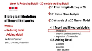
Reduction of Hodgkin-Huxley Model to 2D Neuron Dynamics
Transition from the intricate Hodgkin-Huxley model to simplified 2D neuron dynamics through phase plane analysis, nullclines, and stability of fixed points. Explore the essential elements and principles of neuronal dynamics, including ion channels, action potentials, and neuron models.

Download Presentation

Please find below an Image/Link to download the presentation.
The content on the website is provided AS IS for your information and personal use only. It may not be sold, licensed, or shared on other websites without obtaining consent from the author.If you encounter any issues during the download, it is possible that the publisher has removed the file from their server.
You are allowed to download the files provided on this website for personal or commercial use, subject to the condition that they are used lawfully. All files are the property of their respective owners.
The content on the website is provided AS IS for your information and personal use only. It may not be sold, licensed, or shared on other websites without obtaining consent from the author.
E N D
Presentation Transcript
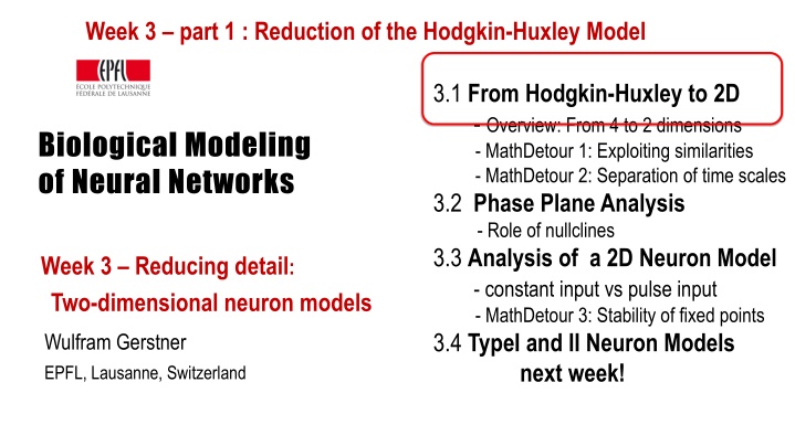
Week 3 part 1 : Reduction of the Hodgkin-Huxley Model 3.1 From Hodgkin-Huxley to 2D - Overview: From 4 to 2 dimensions - MathDetour 1: Exploiting similarities - MathDetour 2: Separation of time scales 3.2 Phase Plane Analysis - Role of nullclines 3.3 Analysis of a 2D Neuron Model - constant input vs pulse input - MathDetour 3: Stability of fixed points 3.4 TypeI and II Neuron Models next week! Biological Modeling of Neural Networks Week 3 Reducing detail: Two-dimensional neuron models Wulfram Gerstner EPFL, Lausanne, Switzerland
Neuronal Dynamics 3.1. Review :Hodgkin-Huxley Model cortical neuron ( ) I t du dt u = ... Hodgkin-Huxley model Compartmental models
Neuronal Dynamics 3.1 Review :Hodgkin-Huxley Model Week 2: Cell membrane contains - ion channels - ion pumps Dendrites (week 4): Active processes? assumption: passive dendrite point neuron spike generation -70mV Na+ action potential K+ Ca2+ Ions/proteins
Neuronal Dynamics 3.1. Review :Hodgkin-Huxley Model inside 100 Ka K mV Na outside 0 Ion channels Ion pump kT q ( ( ) ) n u n u = = ln u u u 1 1 2 2 Reversal potential voltage difference ion pumps concentration difference
Neuronal Dynamics 3.1. Review: Hodgkin-Huxley Model Hodgkin and Huxley, 1952 inside 100 I Ka mV C gK gl gNa Na 0 outside Ion channels Ion pump stimulus I 4 equations = 4D system KI I leak Na du 3 4 = + ( ) ( ) ( ) ( ) C g m h u E g n u E g u E I t Na Na K K l l dt n0(u) h ( ( u ( ) u ) ) dm dn dh m n h m ( u ( u n 0 u = = = (u ) 0 0 u ) n n h ( ) ) dt dt dt m u u
Neuronal Dynamics 3.1. Overviewand aims Can we understand the dynamics of the HH model? - mathematical principle of Action Potential generation? - constant input current vs pulse input? - Types of neuron model (type I and II)? (next week) - threshold behavior? (next week) Reduce from 4 to 2 equations Type I and type II models f-I curve ramp input/ constant input f-I curve f f I0 I0 I0
Neuronal Dynamics 3.1. Overviewand aims Can we understand the dynamics of the HH model? Reduce from 4 to 2 equations
Neuronal Dynamics Quiz 3.1. A - A biophysical point neuron model with 3 ion channels, each with activation and inactivation, has a total number of equations equal to [ ] 3 or [ ] 4 or [ ] 6 or [ ] 7 or [ ] 8 or more
Neuronal Dynamics 3.1. Overviewand aims Toward a two-dimensional neuron model -Reduction of Hodgkin-Huxley to 2 dimension -step 1: separation of time scales -step 2: exploit similarities/correlations
Neuronal Dynamics 3.1. Reductionof Hodgkin-Huxley model stimulus I I I Na leak K du dt= dm = + 3 4 ( ) ( ) ( ) ( ) I t C g m h u E g n u E g u E Na Na K K l l ( ) m m u (u ) m0(u) 0 u ( h ( ) u dt dh m h h0(u) (u ) ) h m = 0 u u ( ) dt u h ( ) dn n n u = 0 u MathDetour ( ) dt n = ( ) ( ( )) m t m u t 1) dynamics of m are fast 0
Neuronal Dynamics MathDetour3.1: Separation of time scales Two coupled differential equations dx dt = + ( ) x c t 1 dx dt dy dt = + ( ) h y x 1 = + ( ) f y ( ) g x 2 Exercise 1 (week 3) (later !) Separation of time scales = ( ) h y x 1 2 Reduced 1-dimensional system dy dt = + ( ) f y ( ( )) g h y 2
Neuronal Dynamics 3.1. Reductionof Hodgkin-Huxley model stimulus I I I Na leak K du dt= dm + 3 4 ( ) ( ) ( ) ( ) I t C g m h u E g n u E g u E Na Na K K l l ( ) m m u (u ) = 0 u n0(u) h ( ) dt n m h0(u) (u ) ( ) h h u dh m = 0 u u ( ) dt u h ( ) dn n n u = 0 u ( ) dt n = ( ) ( ( )) m t m u t 1) dynamics of m are fast 2) dynamics of h and n are similar 0
Neuronal Dynamics 3.1. Reductionof Hodgkin-Huxley model Reduction of Hodgkin-Huxley Model to 2 Dimension -step 1: separation of time scales -step 2: exploit similarities/correlations Now !
Neuronal Dynamics 3.1. Reductionof Hodgkin-Huxley model stimulus du dt= + 3 4 ( ) ( ) ( ) ( ) I t C g m h u E g n u E g u E Na Na K K l l = 1 ( ) ( ) h t a n t 2) dynamics of h and n are similar MathDetour u t 1 h(t) n(t) hrest nrest 0 t
Neuronal Dynamics Detour3.1. Exploit similarities/correlations dynamics of h and n are similar h = 1 ( ) ( ) h t a n t 1-h Math. argument n 1 h(t) n(t) hrest nrest 0 t
Neuronal Dynamics Detour3.1. Exploit similarities/correlations dynamics of h and n are similar = 1 ( ) ( ) h t a n t at rest ( ) h h u dh n = 0 u ( ) dt h 1 ( ) dn n n u h(t) n(t) hrest = 0 u nrest ( ) dt n 0 t
Neuronal Dynamics Detour3.1. Exploit similarities/correlations dynamics of h and n are similar (i) Rotate coordinate system (ii) Suppress one coordinate (iii) Express dynamics in new variable = = 1 ( ) ( ) ( ) h t an t w t ( ) h h u dh n = 0( ) ( ) u w w u dw dt 0 u = ( ) dt h 1 eff ( ) dn n n u h(t) n(t) hrest = 0 u ( ) nrest dt n 0 t
Neuronal Dynamics 3.1. Reductionof Hodgkin-Huxley model I I I leak K Na du dt = + 3 4 [ ( )] ( )( ( ) m t h t u t ) [ ( )] ( ( ) n t ) ( ( ) g u t ) ( ) I t C g E g u t E E Na Na K K l l du dt w = + 3 4 0( ) (1 m u )( ) [ ] ( a ) ( ) ( ) I t C g w u E g u E g u E Na Na K K l l = ( t ( ) h ( a ( )) ) t 1) dynamics of m are fast 2) dynamics of h and n are similar m 1 t m ) u t ( 0 = n w(t) w(t) ( ) h h u dh = 0 u 0( ) ( ) u w w u dw dt ( ) dt = h ( ) dn n n u = 0 u eff ( ) dt n
Neuronal Dynamics 3.1. Reductionof Hodgkin-Huxley model K I I I Na leak du dt w = + 3 4 0( ) (1 m u )( ) ( ) ( a ) ( ) ( ) I t C g w u E g u E g u E Na Na K K l l 0( ) ( ) u w w u dw dt = eff du dt dw dt = + ( ( ), ( )) F u t w t ( ) RI t = ( ( ), ( )) G u t w t w
NOW Exercise 1.1-1.4: separation of time scales du dt= + 3 4 ( ) ( ) ( ) ( ) I t C g m h u E g n u E g u E Na Na K K l l (t ) c ( ) dm m m u (t ) dx x c = 0 u = ( ) dt dt A: - calculate x(t)! - what if is small? m 0 1 t (t ) x Exercises: 1.1-1.4 now! 1.5 homework ? t ( ) dm m c u Exerc. 9h50-10h00 Next lecture: 10h15 B: -calculate m(t) if is small! - reduce to 1 eq. = dt du m = ( ) f u m dt
Week 3 part 1 : Reduction of the Hodgkin-Huxley Model 3.1 From Hodgkin-Huxley to 2D - Overview: From 4 to 2 dimensions - MathDetour 1: Exploiting similarities - MathDetour 2: Separation of time scales 3.2 Phase Plane Analysis - Role of nullclines 3.3 Analysis of a 2D Neuron Model - constant input vs pulse input - MathDetour 3: Stability of fixed points 3.4 TypeI and II Neuron Models next week! Biological Modeling of Neural Networks Week 3 Reducing detail: Two-dimensional neuron models Wulfram Gerstner EPFL, Lausanne, Switzerland
Neuronal Dynamics MathDetour3.1: Separation of time scales Two coupled differential equations dx dt dx dt dy dt Ex. 1-A = + ( ) x c t = + ( ) x c t 1 1 = + ( ) f y ( ) g x 2 Exercise 1 (week 3) Separation of time scales 1 2 Reduced 1-dimensional system dy dt = + ( ) f y ( ( )) g c t 2
Neuronal Dynamics MathDetour3.2: Separation of time scales dx dt = + ( ) x c t Linear differential equation 1 step
Neuronal Dynamics MathDetour3.2 Separation of time scales Two coupled differential equations dx dt dc dt x = + ( ) x c t 1 = + ( ) I t + ( ) f x c 2 c 1 2 slow drive I
Neuronal Dynamics Reductionof Hodgkin-Huxley model stimulus I I I Na leak K du dt= dm + 3 4 ( ) ( ) ( ) ( ) I t C g m h u E g n u E g u E Na Na K K l l ( ) m m u (u ) = 0 u n0(u) h ( ) dt n m h0(u) (u ) ( ) h h u dh m = 0 u u ( ) dt u h ( ) dn n n u = 0 u ( ) dt n = ( ) ( ( )) m t m u t dynamics of m is fast 0 Fast compared to what?
Neuronal Dynamics MathDetour3.2: Separation of time scales Two coupled differential equations dx dt dy dt = + ( ) h y x 1 = + ( ) f y ( ) g x 2 Exercise 1 (week 3) Separation of time scales = ( ) h y x even more general 1 2 Reduced 1-dimensional system dy dt = + ( ) f y ( ( )) g h y 2
Neuronal Dynamics Quiz 3.2. A- Separation of time scales: We start with two equations dx x y I t dt dy y x A dt = + + ( ) 1 Attention I(t) can move rapidly, therefore choice [1] not correct = + + 2 2 [ ] If then the system can be reduded to dy y y dt 1 2 = + + + 2 [ ( )] I t A 2 [ ] If then the system can be reduded to dx x x dt 2 1 = + + A I t + 2 ( ) 1 [ ] None of the above is correct.
Neuronal Dynamics Quiz 3.2-similar dynamics Exploiting similarities: A sufficient condition to replace two gating variables r,s by a single gating variable w is [ ] Both r and s have the same time constant (as a function of u) [ ] Both r and s have the same activation function [ ] Both r and s have the same time constant (as a function of u) AND the same activation function [ ] Both r and s have the same time constant (as a function of u) AND activation functions that are identical after some additive rescaling [ ] Both r and s have the same time constant (as a function of u) AND activation functions that are identical after some multiplicative rescaling
Neuronal Dynamics 3.1. Reductionto 2 dimensions 2-dimensional equation du dt dw dt = + ( ( ), ( )) f u t w t ( ) I t C = ( ( ), ( )) g u t w t Enables graphical analysis! Phase plane analysis -Discussion of threshold - Constant input current vs pulse input -Type I and II - Repetitive firing
Week 3 part 1 : Reduction of the Hodgkin-Huxley Model 3.1 From Hodgkin-Huxley to 2D - Overview: From 4 to 2 dimensions - MathDetour 1: Exploiting similarities - MathDetour 2: Separation of time scales 3.2 Phase Plane Analysis - Role of nullclines 3.3 Analysis of a 2D Neuron Model - constant input vs pulse input - MathDetour 3: Stability of fixed points 3.4 TypeI and II Neuron Models next week! Biological Modeling of Neural Networks Week 3 Reducing detail: Two-dimensional neuron models Wulfram Gerstner EPFL, Lausanne, Switzerland
Neuronal Dynamics 3.2. Reduced Hodgkin-Huxley model K I I I Na leak du dt w = + 3 4 0( ) (1 m u )( ) ( ) ( a ) ( ) ( ) I t C g w u E g u E g u E Na Na K K l l ( ) w w u dw 0 u = ( ) dt w stimulus du dt dw w = + ( , ) F u w ( ) RI t = ( , ) G u w dt
Neuronal Dynamics 3.2. PhasePlane Analysis/nullclines 2-dimensional equation stimulus du dt dw = + ( , ) F u w ( ) RI t = ( , ) G u w w dt Enables graphical analysis! -Discussion of threshold -Type I and II u-nullcline w-nullcline
Neuronal Dynamics 3.2. FitzHugh-NagumoModel du dt = + ( , ) F u w ( ) RI t 1 3 = + MathAnalysis, blackboard 3 ( ) u u w RI t dw dt = = + ( , ) G u w b bu w 0 1 w u-nullcline w-nullcline
Neuronal Dynamics 3.2. flowarrows du dt dw w Stimulus I=0 = + dw ( , ) F u w ( ) RI t = 0 dt w = ( , ) G u w dt Consider change in small time step u Flow on nullcline I(t)=0 du = 0 dt Flow in regions between nullclines Stable fixed point
Neuronal Dynamics Quiz 3.3 A. u-Nullclines [ ] On the u-nullcline, arrows are always vertical [ ] On the u-nullcline, arrows point always vertically upward [ ] On the u-nullcline, arrows are always horizontal [ ] On the u-nullcline, arrows point always to the left [ ] On the u-nullcline, arrows point always to the right Take 1 minute, continue at 10:55 B. w-Nullclines [ ] On the w-nullcline, arrows are always vertical [ ] On the w-nullcline, arrows point always vertically upward [ ] On the w-nullcline, arrows are always horizontal [ ] On the w-nullcline, arrows point always to the left [ ] On the w-nullcline, arrows point always to the right [ ] On the w-nullcline, arrows can point in an arbitrary direction
Neuronal Dynamics 4.2. FitzHugh-NagumoModel du dt = + ( , ) F u w ( ) RI t 1 3 = + 3 ( ) u u RI t dw dt = = + ( , ) G u w b bu w 0 1 w change b1
Neuronal Dynamics 3.2. Nullclinesof reduced HH model dw = 0 dt stimulus du dt dw w = + ( , ) F u w ( ) RI t = ( , ) G u w dt du = 0 dt u-nullcline w-nullcline Stable fixed point
Neuronal Dynamics 3.2. PhasePlane Analysis 2-dimensional equation stimulus du dt = + ( , ) F u w ( ) RI t dw = ( , ) G u w w dt Application to neuron models Enables graphical analysis! Important role of - nullclines - flow arrows
Week 3 part 3: Analysis of a 2D neuron model 3.1 From Hodgkin-Huxley to 2D 3.2 Phase Plane Analysis - Role of nullcline 3.3 Analysis of a 2D Neuron Model - pulse input - constant input -MathDetour 3: Stability of fixed points 3.4 Type I and II Neuron Models (next week)
Neuronal Dynamics 3.3. Analysis of a 2D neuron model 2-dimensional equation stimulus du dt dw = + ( , ) F u w ( ) RI t = ( , ) G u w w dt 2 important input scenarios - Pulse input - Constant input Enables graphical analysis!
Neuronal Dynamics 3.3. 2Dneuron model: Pulse input du dt dw dt = + ( , ) F u w RI = ( , ) G u w w pulse input
Neuronal Dynamics 3.3. FitzHugh-NagumoModel : Pulse input 1 3 du dt dw = + = + 3 ( , ) F u w ( ) ( ) RI t u u w RI t = 0 dt w I(t)=0 dw dt = = + ( , ) G u w b bu w 0 1 w u I(t) Pulse input: jump of voltage du pulse input = 0 dt
Neuronal Dynamics 3.3. FitzHugh-NagumoModel : Pulse input = = 0.9; 1.0 FN model with 0 b b Image: Neuronal Dynamics, Gerstner et al., Cambridge Univ. Press (2014) 1 Pulse input: jump of voltage/initial condition
Neuronal Dynamics 3.3. FitzHugh-NagumoModel dw DONE! Pulse input: - jump of voltage - new initial condition - spike generation for large input pulses 2 important input scenarios = 0 dt w I(t)=0 constant input: - graphics? - spikes? - repetitive firing? u Now du = 0 dt
Neuronal Dynamics 3.3. FitzHugh-NagumoModel: Constant input du dt = + ( , ) F u w RI dw w-nullcline w 0 = 0 dt 1 3 = + 3 u u w RI 0 dw dt = = + ( , ) G u w b bu w 0 1 w I(t)=I0 u Intersection point (fixed point) -moves -changes Stability du = 0 dt u-nullcline
NOW Exercise 2.1: Stability of Fixed Point in 2D du dt dw dt = u w dw = 0 dt w = u w - calculate stability - compare Exercises: 2.1now! 2.2 homework I(t)=I0 dx dt x = u du = 0 Next lecture: 11:42 dt
Week 3 part 3: Analysis of a 2D neuron model 3.1 From Hodgkin-Huxley to 2D 3.2 Phase Plane Analysis - Role of nullcline 3.3 Analysis of a 2D Neuron Model - pulse input - constant input -MathDetour 3: Stability of fixed points 3.4 Type I and II Neuron Models (next week)
Neuronal Dynamics Detour 3.3 : Stability of fixed points. dw dt = + b bu w 0 1 w w dw w-nullcline = 0 dt stable? I(t)=I0 u du du dt = 0 = + ( , ) F u w RI dt 0 u-nullcline
Neuronal Dynamics 3.3 Detour. Stability of fixed points 2-dimensional equation stimulus du dt dw = + ( , ) F u w RI 0 = ( , ) G u w w dt How to determine stability of fixed point?
Neuronal Dynamics 3.3 Detour. Stability of fixed points dw = 0 stimulus dt w du = + au w 0 I dt dw = c u w w dt I(t)=I0 u du = 0 dt unstable saddle stable