Regression and OLS Estimation - Parameters, Properties, Tests
This chapter delves into Ordinary Least Squares (OLS) estimation for parameter estimation, exploring the properties of OLS, conducting hypothesis tests on OLS coefficients, and determining confidence intervals. It covers simple economic models, random components, observed factors, and provides examples to illustrate key concepts in regression analysis.
Download Presentation

Please find below an Image/Link to download the presentation.
The content on the website is provided AS IS for your information and personal use only. It may not be sold, licensed, or shared on other websites without obtaining consent from the author.If you encounter any issues during the download, it is possible that the publisher has removed the file from their server.
You are allowed to download the files provided on this website for personal or commercial use, subject to the condition that they are used lawfully. All files are the property of their respective owners.
The content on the website is provided AS IS for your information and personal use only. It may not be sold, licensed, or shared on other websites without obtaining consent from the author.
E N D
Presentation Transcript
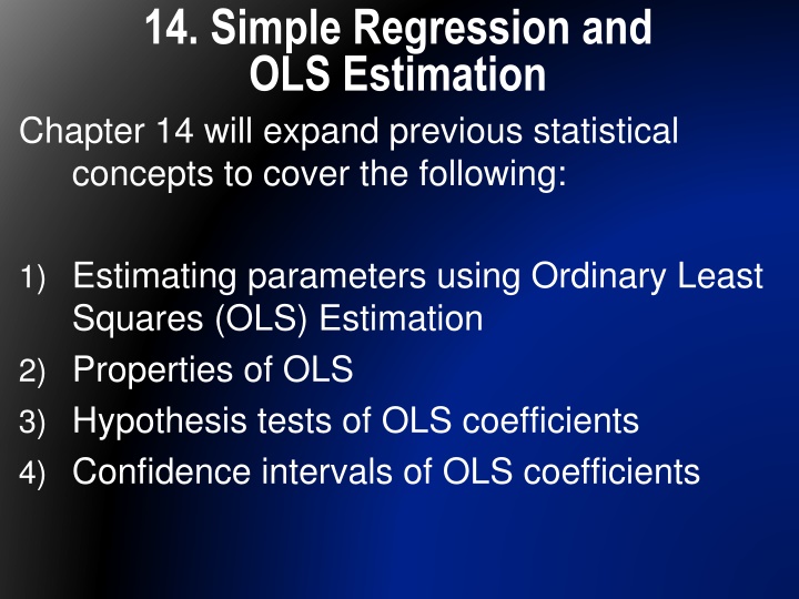
14. Simple Regression and OLS Estimation Chapter 14 will expand previous statistical concepts to cover the following: 1) Estimating parameters using Ordinary Least Squares (OLS) Estimation 2) Properties of OLS 3) Hypothesis tests of OLS coefficients 4) Confidence intervals of OLS coefficients
14. Regression & OLS 14.0 Linear Economic Models 14.1 Regressions 14.2 OLS 14.X OLS Properties 14.? OLS Expanded Predicted Values (14.X) Estimated Errors (14.8) Confidence Intervals (14.6) Hypothesis Tests (14.5) 2
14.0 Simple Economic Models and Random Components Consider the linear economic model: Yi = 1 + 2Xi + i The variable Y is related to another variable X Utility is related to hours of TV watched i (or epsilon) represents error; everything included in Y that is not explained by X Ie: Quality of TV show, Quality of Popcorn, Other Facts of Life 3
14.0 Simple Economic Models and Random Components Consider the linear economic model: Yi = 1 + 2Xi + i This is the TRUE, population relationship between X and Y 1 is the value of Y when X is zero 2 is how much Y increases when X increases by 1 If X and Y are unrelated, 2 is zero 4
14.0 Observed or Random Components i (or epsilon) is the RANDOM ERROR TERM; it takes on values according to chance Since Yi depends on i, it is also random 1 + 2Xi is assumed to be fixed in most simple models (which simplifies everything) Referred to as the deterministic part of the model X, 1 and 2 areNon-Random 1 and 2 are unknown, and must be estimated 5
14.0 Example Consider the function: Utilityi = 1 + 2Sistersi + i Happiness depends on the number of sisters i captures: number of brothers, income, and other factors (ie: bad data collection and shocks) Utility and Sisters are Observable Utility and i are random 1 and 2 must be estimated (< or > 0?) Note: Some texts use 0 and 1 as our unknown variables 6
14.1 What does OLS do? Ordinary Least Squares (OLS) estimation is a regression that creates the best straight line going through the middle of the data points: Studying and Marks 8 7 6 Studying 5 4 3 2 1 0 0 20 40 60 80 100 120 Marks 7
14.2 Estimator Review Population Expected Value: = E(Y) = y f(y) Sample Mean: = Y i Y N __ Note: From this point on, Y may be expressed as Ybar (or any other variable - ie:Xbar). For example, via email no equation editor is available, so answers may be in this format. 8
14.2 Estimator Review Tom and Rodney both go to a 4-day gaming convention. How much they spend (S)each day is listed below: Day 1 2 3 4 Tom 110 85 90 135 Rodney 190 20 10 200 T S + + + 110 85 90 135 4 190 20 10 200 4 T i = = = 105 S N R S + + + R i = = = 105 S N 9
14.2 OLS Population Regression Function: Yi = 1 + 2Xi + i Estimated Regression Function: Y 1 + = X 2 i i 10
14.2 OLS OLS Estimation: ( )( ) X X Y Y i i = 2 2 ( ) X X i ( , ) Cov X 2 Y = 2 S X = Y X 1 2 Note: B2 may be expressed as b2hat ^ 11
14.2 OLS = + Tom t Rodney t S S S 1 1 , T R ( ) 2133 10,833 Cov S = = = 0.197 2 2 R S = = 105 0.197(105) = T R 84.3 S S 1 2 + = Tom t Rodney t 84.3 0.197 S S Note: Although mathematically there is a relationship between Tom and Rodney s spending, in reality there is no connection both are influenced by a 3rd variable the fact that most people spend the most on the first and last day of the convention. 12
14.2 OLS Example 2 Given the data set: Price 4 3 3 6 Quantity 10 15 20 15 Find sample means, variance, covariance, correlation, and ols estimation 13
14.2 OLS Example 2 Price 4 3 3 6 Quantity 10 15 20 15 Sample Means: Pbar = (4+3+3+6)/4 = 4 Qbar = (10+15+20+15)/4 = 15 14
14.2 OLS Example 2 Price 4 3 3 6 Pbar = 4 Quantity 10 15 20 15 Qbar=15 Sample Variance: Sp2 = [(4-4)2+(3-4)2+(3-4)2+(6-4)2]/(N-1) =(0+1+1+4)/3 =2 Sq2 = [(10-15)2+(15-15)2+(20-15)2+(15-15)2]/(N-1) =(25+0+25+0)/3 =50/3 15
14.2 OLS Example 2 Price 4 3 3 6 Pbar = 4 Quantity 10 15 20 15 Qbar=15 Sample Covariance: Cov(p,q)= [(4-4)(10-15)+(3-4)(15-15) +(3-4)(20-15)+(6-4)(15-15)]/(N-1) =[ 0 + 0 -5 +0] /3 = -5/3 16
14.2 OLS Example 2 Price 4 3 3 6 Pbar = 4 Quantity 10 15 20 15 Qbar=15 Sample Correlation Corr(p,q) = Cov(p,q)/SpSq = 5/3 / [2(50/3)]1/2 = -5/3 / (10/31/2) = -0.2886 17
14.2 OLS Example 2 Price 4 3 3 6 Pbar = 4 Quantity 10 15 20 15 Qbar=15 Ols Estimation B2hat = (Xi-Xbar)(Yi-Ybar) ---------------------- (Xi-Xbar)2 = [(4-4)(10-15)+(3-4)(15-15)+(3-4)(20-15)+(6-4)(15-15) ----------------------------------------------------------------------------- (4-4)2+(3-4)2+(3-4)2+(6-4)2 =-5/6 18
14.2 OLS Example 2 Price 4 3 3 6 Pbar = 4 Quantity 10 15 20 15 Qbar=15 Ols Estimation B1hat = Ybar (B2hat)(Xbar) = 15- (-5/6)4 = 90/6 + 20/6 = 110/6 110 5 = Y X i i 6 6 110 5 Q = P i i 6 6 19
14.X Properties of the OLS Estimator There exist a variety of methods to estimate the coefficients of our model ( 1 and 2) Why use Ordinary Least Squares (OLS)? OLS minimizes the sum of squared errors, creating a line that fits best with the observations With certain assumptions, OLS exhibits beneficial statistical properties. In particular, OLS is BLUE. 1) 2) 20
14.X The OLS Estimator and its Properties We ve seen the true economic relationship: Yi = 1 + 2Xi + i Where i and therefore Yi are random and the other terms are non-random When this relationship is unknown, we ve seen how to estimate the relationship Y = + X 1 2 i i N Using: = ( )( ) X X Y Y i i ( , ) Cov X 2 Y = = 1 i 2 N S = 2 ( ) X X X i 1 i = Y X 21 1 2
14.X Fitted or Predicted Values From this OLS example we see that often the actual data points lie above or below the estimated line. Studying and Marks 8 7 6 Studying 5 4 3 2 1 0 0 20 40 60 80 100 120 Marks Points on the line give us ESTIMATED y values for each given x. The predicted or fitted y values are found using our x data and our estimated s: Y 1 + = X 2 i i 22
14.X Estimators Example 4 3 3 Price 6 Pbar = 4 Quantity 10 15 20 15 Qbar=15 Ols Estimation 18 = Q i = 18 3 . . 0 833 Q P 3 . . 0 833 P i i i = 14 9 . Q = = 1 18 3 . . 0 833 Q P 18 3 . . 0 833 Q P 3 3 1 1 = 15 8 . Q = = 18 3 . . 0 833 ) 3 ( 2 18 3 . . 0 833 ) 4 ( Q Q 3 1 = 15 8 . Q = = 14 9 . 15 8 . Q Q 3 1 3 = 13 3 . Q = = 18 3 . . 0 833 18 3 . . 0 833 Q P Q P 4 2 2 4 4 = = 18 3 . . 0 833 ) 3 ( 18 3 . . 0 833 ) 6 ( Q Q 2 4 = = 15 8 . 13 3 . Q Q 23 2 4
14.8 Estimating Errors or Residuals The estimated y values (yhat) are rarely equal to their actual values (y). The difference is the estimated error (or residual): Y E i i = Y Since we are indifferent whether our estimates are above or below the actual, we can square these estimated errors. A higher squared error means an estimate farther from the actual 24
14.8 Estimators Example 4 3 3 Price 6 Pbar = 4 Quantity 10 15 20 15 Qbar=15 = = E Q Q E Q Q i i i i i i = = E Q Q E Q Q 3 3 3 1 1 1 = = 20 15 8 . E 10 14 9 . E 3 1 = = 9 . 4 2 . 4 E E 3 1 = = E Q Q E Q Q 4 4 4 2 2 2 = = 15 13 3 . E 15 15 8 . E 4 2 7 . 1 = = 8 . 0 E E 4 2 25
14.3 SSE A common calculation used in regression analysis is the sum of the squared errors, or SSE: ??? = (?? ?)2 2 ??? = ?? This calculation will be useful in R2 later in the chapter. 26
14.X Statistical Properties of OLS In our model: Y, the dependent variable, is made up of two components: 1 + 2Xi a non-random component that indicates the effect of X on Y. In this course, X is non-random. i a random error term representing other influences on Y. a) b) 27
14.4 Statistical Properties of OLS Error Assumptions: a) E( i) = 0; we expect no error; we assume the model is complete b) Var( i) = 2; the error term has a constant variance c) Cov( i, j) = 0; error terms from two different observations are uncorrelated (independent). If the last error was positive, the next error need not be negative. 28
14.X Statistical Properties of OLS OLS Estimators are Random Variables: a) Y depends on and is thus random. b) 1hat and 2hat depend on Y c) Therefore they are random d) All random variables have probability distributions, expected values, and variances e) These characteristics give rise to certain OLS estimator properties. 29
14.X OLS is BLUE We use Ordinary Least Squares estimation because, given certain assumptions, it is BLUE: B est L inear Unbiased E stimator 30
14.X U nbiased An estimator is unbiased if it expects the true value: E(dhat) = d 2hat = (Xi-Xbar)(Yi-Ybar) ---------------------- (Xi-Xbar)2 2hat = (Xi-Xbar)(Yi) ------------------- (Xi-Xbar)Xi By a mathematical property. 31
14.X U nbiased 2hat = (Xi-Xbar)(Yi) ------------------- (Xi-Xbar)Xi E( 2hat) = (Xi-Xbar)E(Yi) ------------------- (Xi-Xbar)Xi Since only Yi is variable. 32
14.X U nbiased E( 2hat) = (Xi-Xbar)E( 1 + 2Xi+ i) ---------------------------------- (Xi-Xbar)Xi Since Yi = 1 + 2Xi+ i E( 2hat) = (Xi-Xbar)( 1 + 2Xi + 0) ---------------------------------- (Xi-Xbar)Xi Since 1, 2, and Xi are non-random and E( i)=0. 33
14.X U nbiased E( 2hat) = 1 (Xi-Xbar) + 2 (Xi-Xbar)Xi ----------------------------------------- (Xi-Xbar)Xi By simple algebra. E( 2hat) = 1 (Xi-Xbar) + 2 (Xi-Xbar)Xi ----------------- -------------------- (Xi-Xbar)Xi (Xi-Xbar)Xi Since there exists a common denominator. 34
14.X U nbiased E( 2hat) = 1(0) + 2 --------------- (Xi-Xbar)Xi Since the sum of the difference between an observation and its mean is zero, by definition, E( 2hat) = 0 + 2 = 2 The proof that E( 1hat)= 1 is similar. 35
14.X U nbiased E( 2hat) = 2 This means that on average, OLS estimation will estimate the correct coefficients. Definition: If the expected value of an estimator is equal to the parameter that it is being used to estimate, the estimator is unbiased. 36
14.X L inear The OLS estimators are linear in the dependent variable (Y): -Y s are never raised to a power other than 1 -no non-linear operations are performed on the Y s Note: Since X s are squared in the 1hat and 2hat formulae, OLS is not linear in the X s (which doesn t matter for BLUE) 37
14.X B est Of all linear unbiased estimators, OLS has the smallest variance. -there is a greater likelihood of obtaining an estimate close to the actual parameter Large variance => High probability of obtaining an estimate far from the center Small variance => Low probability of obtaining an estimate far from the center 38
14.X E stimator By definition, the OLS estimator is an estimator; it estimates values for 1 and 2. 39
14.X Normality of Y In order to conduct hypothesis tests and construct confidence intervals from OLS, we need to know the exact distributions of 1hat and 2hat (Otherwise, we can t use statistical tables..) We will see that if 1) The error term is normally distributed Then 2) Y is normally distributed Then 3) 1hat and 2hat are normally distributed
14.4 Normality of Y So far, we have assumed: The error term, i, is random with E( i)=0; no expected error Var( i)= 2; constant variance Cov( i, j)=0; no covariance between errors Now we add the assumption that the error term is normally distributed. Therefore: iid i ~ N(0, 2) (iid means identically and independently distributed)
14.X Normality of Y If the error is normally distributed, so will be the Y term (since the randomness of Y depends on the randomness of the error term). Therefore: E(Yi) = E( 1+ 2Xi+ i)= 1+ 2Xi Var(Yi) = Var( 1+ 2Xi+ i)=Var( i) = 2 (Given all our previous assumptions.) Therefore: Yi ~ N( 1+ 2Xi, 2) (Y is normally distributed with mean 1+ 2Xi and variance 2.)
14.X Normality of OLS Since 1hat and 2hat are linear functions of Y: X 2 i X 2 ~ ( , ) N 1 1 2 N ( ) X i 2 ~ ( , ) N 2 2 2 ( ) X X i
14.X Normality of OLS If we know , we can construct standard normal variables (z=(x- )/ ): 1 1 N X N i ~ ) 1 , 0 ( 2 i 2 2 ( ) X X ~ ) 1 , 0 ( N 2 2 2 2 ( ) X X i
14.X Normality of OLS Since we don t know 2, we can estimate it: N = 2 ei 2 2 This gives us estimates of the variance of our coefficients: = 1 ) r( a v ( X 2 i X 2 N 2 ) X i 2 = a v r( ) 2 2 ( ) X X i
14.X Normality of OLS The square root of the estimated variance is referred to as the standard error (se) (as opposed to standard deviation) Using our assumptions: ( 1hat- 1)/se( 1hat) has a t distribution with N-2 degrees of freedom ( 2hat- 2)/se( 2hat) has a t distribution with N-2 degrees of freedom Note: se of 1hat and 2hat is often part of statistical estimation (such as excel)
14.X OLS and Goodness of Fit On average, OLS works well: The average of the estimated errors is zero = 0 ie The average of the estimated Y s is always the average of the observed Y s Y N i = Y i N
14.X Measuring Goodness of Fit These conditions hold regardless of the quality of the model. Ie: You could estimate average grades as a function of locust population in Mexico. OLS would be a good estimator even though the model is useless. Goodness of Fit measures how well the economic model fits the data. R2 is the most common measure of goodness of fit. R2 CANNOT be compared across models.
14.X Measuring Goodness of Fit R2 is constructed by dividing the variation of Y into two parts: 1) Variation in fitted Yhat terms. This is explained by the model 2) Variation in the estimated errors. This is NOT explained by the model. = = i 1 N N = i 2 2 e ( ) Y Y i i = 2 1 1 1 i R N N = = i 2 2 ( ) ( ) Y Y Y Y i i 1
14.X Measuring Goodness of Fit R2 is the proportion of variation explained by the model. It is expressed as: a) The ratio of explained variation to total variation in Y Or b) 1 minus the ratio of unexplained variation to total variation in Y 0<R2<1 R2=0; model has no explanatory power R2=1; model completely explains variations in Y (and generally that means you did something wrong)
