Explore the Romerian contribution to empirical analysis of economic growth, critiquing convergence literature and discussing models, empirical results, and conclusions. Delve into the determinants of variations in real income across countries, the speed of convergence, and the impact of technological progress on long-run economic growth.
Please find below an Image/Link to download the presentation.
The content on the website is provided AS IS for your information and personal use only. It may not be sold, licensed, or shared on other websites without obtaining consent from the author. If you encounter any issues during the download, it is possible that the publisher has removed the file from their server.
You are allowed to download the files provided on this website for personal or commercial use, subject to the condition that they are used lawfully. All files are the property of their respective owners.
The content on the website is provided AS IS for your information and personal use only. It may not be sold, licensed, or shared on other websites without obtaining consent from the author.
E N D
Presentation Transcript
A Romerian Contribution to the Empirics of Economic Growth Bahar Bayraktar-Sa lam Hacettepe University Hakan Yetkiner Izmir University of Economics At l m University, Ankara May 4, 2012 1
A Critique of Convergence Literature The following equation (or its variations) is used in empirical growth literature in order to designate the determinants of variations in real income across countries (cf., Mankiw, Romer and Weil, (1992) : In the equation above, Initial knowledge stock plus all sources of variations : g Exogenous rate of growth/ technological progress = + + + + [ ] [ 0 ( A )] [ ] [ ] Ln y Ln g t Ln s Ln g n ss 1 1 [A 0 ( )] : Ln We now know that is defined by the characteristics of R&D sector, by and large. g 3
A Critique of Convergence Literature In a similar vein, the following equation (or its variations) is used in identifying the speed of convergence, that is, the rate at which poorer countries tend to grow faster than rich ones and catch them up: Ln v dt = n v ~ y [ ] dLn ] ss ~ y ~ y = [ ] [ Ln + + 1 ( )( ) g ( ) ) 0 ( Y t Y = + vt vt [ ] [ ] 1 ( ) [ 0 ( )] 1 ( ) [ 0 ( )] Ln Ln e Ln A e Ln Y g t ( ) ) 0 ( L t L + + + + vt vt 1 ( ) [ ] 1 ( ) [ ] e Ln s e Ln g n 1 1 4
A Critique of Convergence Literature-I In almost all empirical studies, the exogenous growth rate of technology is taken same across countries and constant in time. This is understandable, as the Solow framework is a one-sector simple model and there is no way to decompose the technological progress into its components. However, it is unrealistic (and unacceptable), as it is the technological progress that determines long-run economic growth and convergence performance (cf. Howitt, 2000). 5
A Critique of Convergence Literature-I Bloom et al. (2002): Object both the idea of identical rate of technological progress in every country and the fixed effects approach adopted by panel data studies, which allow for TFP differentials across countries that persist indefinetely. 6
A Critique of Convergence Literature-II Consider the naivety of adding new components into these equations across the whole empirical literature. The current application is merely to add the variable in question to the growth/ convergence equations. At the best, researchers follow MRW (1992)-type modeling approach and add new accumulation functions. To what extent is this satisfactory? Can we find a more elegant way of introducing additional elements to study the determinants of long run GDP per capita and speed of convergence? 7
A Critique of Convergence Literature-III How about Robustness of MRW (1992) Model? 1 1 L = s vs. = s s ( ) Y K t = K Y H ( ) = = Y t K Y I H K H K H K I Y = H s Y H H H Steady state at levels vs. Endogeneous Growth! 8
A Critique of Convergence Literature-IV Since 1986, thousands of studies have been done in endogenous/ new growth theory, showing the role of endogenous technological change on transtitonal and long run economic growth. On the empirical side, however, we still use the Solow framework and we continue to assume exogenous technological change and exogenous growth rate. Is it impossible to endogenize technological change in such a way that fits empiricalworld ? Though this is not achieved in this paper, this work underlines the need in this direction. 9
Literature (1) Romer (1990): Endogenous Technological Change Solow (1956): Exogenous Technological Change Mankiw, Romer Weil (1992): Solow model is too good to ignore. Islam (1995): Panel data version of MRW (1992) Barro, Sala-i-Martin (1992): Convergence in Ramsey Jones (2002); Kim (2008, 2011) Whelan (2007) 10
Contribution of this paper This paper develops a Romerian Solow Framework/ Solovian Romer Framework/ semi-endogenous growth model and tests it, in which it is possible (i) to decompose the components of exogenous growth rate (ii) to work out a richer and more flexible framework (iii) to extend the framework in several directions (limited only by imagination) (iv) introduce human capital in a more elegant way (v) possibly more robust compared to MRW (1992) 11
General Features of the Model - Solovian Romer model - Factors of production: X (intermediate goods) and L (human capital) - Exogenous determination of consumption-saving tradeoff - Final-goods market is perfectly competitive - Intermediate goods market is monopolistically competitive - R&D sector is perfectly competitive. 12
The model I. Final-Good Production ( ) A t 1 Y = = 0 1 Y H X i 1 i Y: Final Output Xi: Intermediate Good i (Variety i) HY: Human Capital allocated to Y 13
The model II. Human Capital Allocation = + = H H 1 = H H & & R D R D & Y R D Y Y HY HR&D : Human capital allocated to R&D-sector Y : Human capital share of final-good sector R&D : Human capital share of R&D sector : Human capital allocated to final-good sector III. Macroeconomic Budget Constraint: = K s Y K 14
The Model IV. R&D Sector A = H A & R D A HR&D : Human capital allocated to R&D : Stock of Knowledge Using the share definition: A = H A & R D 15
Solution Procedure Profit maximization in the final-good market yields: ( ) A = t = 1 1 x p x = 1 ( ) w Y i Y Y i i 1 i Profit maximization in the intermediate-good market yields: r p pi = = + r = + = r r 1 r 2 1 = = x x i Y 1 a = = 1 1 ( ) r x x i Y H 16
Solution Procedure Final-good and intermediate-good markets profit maximization results imply: ( ) ( ) A = t A = t ( ) ( ) A = t A = t = = = = = = K K X X A k k x x A i i i i 1 1 i i 1 1 i i = = 1 Y 1 1 y x A y k A Y 17
R&D Sector equilibrium process implies: = V H A w = H & & & & & R D R D R D R D w R D V L A & & & R D R D R D The value of patents is found as follows: ( ) r s ds ( ) H t = = ( ) ( ) V t H e d V t t & , & , R D i R D i ( ) r t t 18
Recall that we assumed and are constant. Solving the model under this assumption, we find that R& D Y s 1 ~ y = ss Y + g A = g H & ss R D This is very similar to the Solow-result: s 1 ~ yss = + g A Evidently, much richer in the sense that it decomposes into its components and underlines the role of human capital in final good production in growth. ss 19
Empirical Applications: Long-run determinants of GDP per capita Solovianized Romer version: = + + + + ln ln[ ] ln[ ] ln[ ] y a gt s g ss Y 1 1 A = a [A 0 ( )] Ln g H & ss R D Solow version: = + + + ln ln[ ] ln[ ] yss a g t s g 1 1 a = [A 0 ( )] . 0 02 Ln g 20
Empirical Applications: Convergence Equation Solovianized Romer version: ( ) ) 0 ( ) 0 ( Y t Y Y ( ) Y = + Ln Ln Ln Ln 0 1 2 H H H ( ) s ( ) + + Ln Ln g 3 3 ( ) ( ) ) 0 ( A = = = = + e ) t 1 g t e e e Ln 0 : Constant term 1 : Coefficient of initial level of income 2 : Contribution of human capital 3 : Contribution of investment rate 0 ( ( 1 ( 1 ) ) 1 t 1 t 2 t 3 1 21
Empirical Applications: Convergence Equation Solow version : ( ) ) 0 ( ) 0 ( Y t Y Y ( ) s ( ) = + + Ln Ln Ln Ln Ln g 0 1 3 3 H H H 0 : Constant term 1 : Coefficient of initial level of income 3 : Contribution of investment rate Recall that g is not defined in Solow version Therefore, it is taken constant in time and identical across countries. 22
Extensions-1 Generalized Knowledge/ R&D Sector R A = Suppose that H A 0 , 1 & D : Degree of positive externality on current R&D : Duplications/ production elasticity of HR&D n One can show that: Ass =1 1 1 1 s s = k A = y A 1 n ss Y ss 1 n ss Y ss + + n + + n 23
Extensions-1 Generalized Knowledge/ R&D Sector Determinants of long-run growth: 1 1 1 n R 1 ( ) s t 1 = y e & D 1 n ss Y n + + n 1 1 = + + + ln ln[ ] ln[ ] ln[ ] ln[ ] ln[ ] y s g & ss Y R D 1 1 1 1 + + + ln[ ] g n gt 1 n where and =1 g = ) 0 ( H 1 24
Extensions-1 Generalized Knowledge/ R&D Sector Convergence: = R A = 1 1 ss= H A g A n Under and & D Knowledge accumulation in terms of per human capital becomes a = 1 a n a & R D Together with capital accumulation equation ~ 1 = ~ ~ A ( + + ( )) k s k n t k Y We have a two-equation differential equation system 25
Extensions-1 Generalized Knowledge/ R&D Sector Convergence: Solving this system through log-linearization, we get b b ~ + + = + + + 1 ( )( ) n g t nt ( ) Ln k const e const e 1 2 1 2 + + 1 ( )( ) n g n + + 1 ( )( ) n g n b nt = + ~ ( ( ) Ln a const e 2 2 n n = + + + ( ) 1 ( ) ( ) ) ( ) Ln y Ln Ln k Ln a nt Y 26
Extensions-2 Unskilled Labor Next to Skilled Labor ( ) A t = 1 Suppose that Y L H X di 0 Y i L : The constant amount of unskilled labor One can show that: 1 1 L s ~ K 1 = 1 1 Y H ss + g 1 L s ~ Y 1 = 1 1 Y H ss + g 27
Extensions-2 Unskilled Labor Next to Skilled Labor Long-run determinants of economic growth: 1 1 1 Y L H s 1 = A ss Y + + + + L H L H L H g 1 = + + + + [ ] [ ] [ ] Ln y a g t Ln Ln Ln s ss L Y 1 1 1 [ + + ] Ln g 1 L + Y + = = = = a + g H y ss [ 0 ( )] Ln A L ss & R D L H L H 28
Extensions-2 Unskilled Labor Next to Skilled Labor Convergence: ( ) ) 0 ( + ( ) 0 ( + Y t Y Y ( ) ( ) s ( ) = + + + Ln Ln Ln Ln Ln ) 0 1 2 3 L Y + L H L H ) ) 0 ( A L H ( ) + + + Ln Ln g ( t = + 4 5 1 g t e Ln 0 ( ) = ( 1 t 1 e 1 1 ) 1 = t e 2 ( ) = t 1 e ) 3 1 1 ( = t 1 e 4 = 29 5 4
Extensions-3 Endogenous Allocation of Skilled Labor between Y and R&D Long-run determinants of Economic Growth: = + + + + + ln ln[ ] ln[ ] ln[ ] y a g t s g , ss Y SS 1 1 where 1 ( ) + ( ) s H = , Y ss + s H 30
Suitability for Further Extensions-1 Health ( ) A t = i = 1 Y Y N N X L i 1 = = N h L N h H = N h H L L Y Y Y & & & R D R D R D 1 1 Y = + + + + ln ln[ ] ln[ ] ln[ ] ss + a g t h h Y Y L 1 1 1 H L + + + + ln[ ] ln[ ] ln[ ] s g L 1 1 1 31
Suitability for Further Extensions-2 Defense Spending I. The Defense Sector = w H M Y M M M M: Military Expenditure M: tax rate (=share of military expenditure in GDP) (=research intensity in defense sector) wM: Real wage rate of human capital in military sector 32
Suitability for Further Extensions-2 Defense Spending II. Profit Equation ( ) ( ) A t A t = = i = i 1 Y 1 ( ) H x w p x Y M i Y Y i i 1 1 III. Human Capital Allocation = = = H H H H H H Y Y M M & & R D R D + + = 1 & Y R D M 33
Suitability for Further Extensions-2 Defense Spending IV. Macroeconomic Budget Constraint: K = ) 1 ( s Y K M V. R&D Sector A = + 1 ( ) H A & R D M 34
Suitability for Further Extensions-2 Defense Spending Long-run determinants of GDP per capita = + + + + + + ln ln[ ] ln[ ] ln[ 1 ] ln[ ] y a g t s g ss Y M 1 1 1 = 1 ( + ) = a + g H [ 0 ( )] Ln A & R D M 35
Empirical Applications: Long-run determinants of GDP per capita for developing Countries (No Spillover Effect) = w L M Y Balanced Budget M M = + + + + + + ln ln[ ] ln[ ] ln[ 1 ] ln[ ] y a g t s g ss Y M 1 1 1 + & = D = 1 g H = a + [ 0 ( )] Ln A Y R & R D 36
Suitability for Further Extensions-2 Defense Spending Convergence Equation ( ) ) 0 ( ) 0 ( Y t Y Y ( ) Y ( ) s = + + + Ln Ln Ln Ln Ln 0 1 2 3 H H H ( ) ( ) + + + 1 Ln Ln g 4 5 M ( ) ( ) ) 0 ( A = = = = + e ) t 1 g t e = e Ln 0 : Constant term 1 : Coefficient of initial level of income 2 : Contribution of human capital 3 : Contribution of investment rate 4 : Contribution of defense intensity 5 : Contribution of effective depreciation rate 0 ( ( 1 ) 1 t 1 ( t 2 ) t 1 e 3 4 1 = 5 4 37
Testing the Model (1) Following MRW 1992, empirical growth studies have estimated an augmented Solow model by assuming the (exogenous) technology growth rate, g, to be a constant value. Even studies like Nonneman and Vanhoudt (1996), Murthy and Chien (1997) and Keller and Poutvaara (2005), using the augmented Solow model to test for the role of technological know-how on economic growth and convergence, assumed that the exogenous technology parameter, g, is constant and be 0.02, as in the vein of the MRW 1992. One first and foremost empirical contribution of this paper is dropping this assumption, based on our theoretical results. We determined g through using the share of R&D personnel in the labor force/ share of R&D expenditure in GDP. 39
Testing the Model (2) This paper, to the best of our knowledge, is also the first which estimates the convergence equation by defining the technological progress as a function of the share of R&D personnel in the labor force. Our first empirical run replaces the constant technology growth by the share of R&D personnel in the labor force, which differs across countries and time. Second empirical run (testing sensitivity of the model) replaces the constant technology growth by the share of R&D expenditure in GDP 40
Testing the Model (3) Variables and sources of data: Variable ( ) y Ln Definition Logarithm of growth in real GDP per head of population aged 15-64 years expressed in 2000 purchasing power parities logarithm of lagged growth in real GDP per head of population aged 15-64 years expressed in 2000 purchasing power parities Gross fixed investment share of GDP Secondary school enrollment rate The share of final good workers in the labor force. Data Source OECD Accounts Annual National ( ) OECD Accounts Annual National Ln ty 1 ( ) s ( ) 1 ( ) 2 ( R ( R World Development Indicators Database Barro-Lee Education Dataset (2010) Own calculations 1 & = + D R Y OECD Main Technology Indicators database OECD Main Technology Indicators database Ln Ln h where Ln h ) ) The share of R&D in the labor force The share of R&D expenditure on GDP Science and & D Ln 1 Science and & D Ln 2 41
Testing the Model (4) Basic statistics: Variables Mean Standard Min Max Deviation 8858 3.8 Real GDP per capita 21291 22.8 5326 17 62731 37 Share of Investment in GDP Secondary Enrollment rates 45.6 13.9 8.2 88 The share of R&D personnel 4.9 2.68 0.44 15 in the labor force The share of R&D 1.56 0.83 0.2 3.9 expenditure in GDP The population growth rate 0.65 0.68 -0.4 6 (%) 42
Testing the Model (5) The equation estimated: y ln ln = + ln ln y y s 1 1 1 2 it it it it + + + + ln ln[ ] h n g 3 4 it it it + + + i t it 43
Testing the Model (6) Methodology: System GMM estimation proposed by Arellano and Bover (1995) and Blundell and Bond (1998) (Stata 10 is used for analyses). Advantages of the System GMM 1. It provides consistent estimates in the presence of Measurement error Endogenous regressors 2. It is highly recommended for the empirical growth studies (Bond etal., 2001). To check for the validity of the instruments, we carried out Hansen Test and serial correlation (M2) test and they approve the validity of instruments. 44
Findings (2): The share of R&D expenditure over GDP Dependent Variable: log differences in GDP per working person OLS OLS Within Group 2.1698*** (0.427) Within Group 2.015*** (0.417) System GMM System GMM Constant -0.089 (0.387) -0.084 (0.402) 0.299 (0.577) 0.645 (0.542) ( ) -0.023*** (0.038) -0.032*** (0.042) -0.2784*** (0.031) -0.2749*** (0.032) -0.097*** (0.107) -0.1539*** (0.064) Ln y 1 it ( ) it ( ) it + g 0.133** (0.063) 0.123** (0.059) 0.030 (0.020) 0.007 (0.025) 0.245*** (0.066) 0.243*** (0.067) 0.031 (0023) -0.040 (0.037) 0.222*** (0.058) 0.190*** (0.060) 0.085** (0.032) 0.081* (0.042) Ln s Ln h ( ) + 0.005 (0.024) -0.043 (0.036) 0.056 (0.038)* n Ln it it 2 0.97 0.97 0.94 0.94 R Implied 0.0008 0.001 0.011 0.011 0.003 0.005 Number of Observations Number of Groups Number of Instruments Hansen test p value Difference Hansen p value M2 150 150 150 30 150 30 150 30 20 0.10 0.06 0.837 150 30 21 0.15 0.06 0.845 46
Findings (3) 1.All runs imply a convergence rate lower than that which is suggested by the literature in general. 2. The investment rate has a positive and statistically significant contribution to convergence in all runs. 3. The role of human capital on convergence is positive but statistically insignificant according to the OLS and Within Group estimators. But, human capital has significant and positive impact on economic growth once the regressions are carried out by the system GMM, where the system GMM estimates are more efficient than the once obtained by the OLS and Within Group estimators (Bond et al., 2001). 47
Findings (4) 4. The sum of population growth and the technology growth, which is proxied by the share of R&D workers in the labor force, and the constant depreciation rate has a positive and statistically significant impact on economic growth according to the system GMM estimation. 48
Findings (5) To check for the consistency of the results, we also replicate the basic MRW (1992) model with human capital accumulation . The estimation of the model, under the assumption of exogenous growth rate of technology, finds a convergence rate to be 0.02. But, once the intensity is substituted for the growth rate of technology, the estimation of the model reveals a lower convergence rate, namely, 0.01. g (the growth rate of technology) 0.02 R&D intensity 0.01 Implied 0.02 49
Conclusion The Solovian growth framework, which is widely used in empirical studies has two weaknesses: exogenous growth rate is undefined and is not suitable for theoretical extension. Romerian Solow framework is a good candidate for overcoming these weaknesses because: (i) it allows for theory-backed extensions for empirical work, (ii) The framework yields conservative convergence rate results, which is intuitive (iii)the determinants of the exogenous growth rate is unveiled. 50


")


")
")
")
")
")
")
: The share of labor devoted to R&D")
: The share of R&D expenditure over GDP")
")
")
")