Sampling Theorem in Signal Processing: Representation and Reconstruction

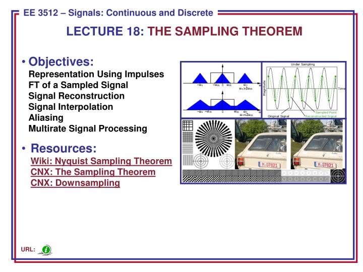
ECE 8443 Pattern Recognition EE 3512 Signals: Continuous and Discrete LECTURE 18: THE SAMPLING THEOREM Objectives: Representation Using Impulses FT of a Sampled Signal Signal Reconstruction Signal Interpolation Aliasing Multirate Signal Processing Resources: Wiki: Nyquist Sampling Theorem CNX: The Sampling Theorem CNX: Downsampling URL:

Representation of a CT Signal Using Impulse Functions The goal of this lecture is to convince you that bandlimited CT signals, when sampled properly, can be represented as discrete-time signals with NO loss of information. This remarkable result is known as the Sampling Theorem. x(t) Recall our expression for a pulse train: = n = ( ) ( ) p t t nT t -2T -T 0 T 2T A sampled version of a CT signal, x(t), is: = n ( ) ( ) = n = = ) = ) ( ) ( ) ( ) ( ( x t x t p t x t t nT x nT t nT s This is known as idealized sampling. We can derive the complex Fourier series of a pulse train: = k = = jk t ( ) where 2 / p t c e T 0 0 k / 2 / 2 T T 1 1 1 1 T T = = = = jk t jk t jk t ( ) ( ) c p t e dt t e dt e 0 0 0 = 0 t k T T T T / 2 / 2 1 = k = jk t ( ) p t e 0 T EE 3512: Lecture 18, Slide 1

Fourier Transform of a Sampled Signal The Fourier series of our sampled signal, xs(t) is: = k T 1 = = jk t ( ) ( ) ( ) ( ) x t p t x t x t e 0 s Recalling the Fourier transform properties of linearity (the transform of a sum is the sum of the transforms) and modulation (multiplication by a complex exponential produces a shift in the frequency domain), we can write an expression for the Fourier transform of our sampled signal: ( = k T 1 ) ( 0 ) 1 1 = k = = = jk t jk t j F F F ( ) ( ) ( ) ( ) X e p t x t x t e x t e 0 0 s T = k = j k ( ) X e T = j If our original signal, x(t), is bandlimited: ( ) 0 for X e B EE 3512: Lecture 18, Slide 2

Signal Reconstruction ( ) j 2 B Note that if , the replicas of do not overlap in the frequency domain. We can recover the original signal exactly. X e s = The sampling frequency, , is referred to as the Nyquist sampling frequency. 2 B s There are two practical problems associated with this approach: The lowpass filter is not physically realizable. Why? The input signal is typically not bandlimited. Explain. EE 3512: Lecture 18, Slide 3

Signal Interpolation The frequency response of the lowpass, or interpolation, filter is: = elsewhere , 0 , T B B j ( ) H e The impulse response of this filter is given by: ( ) ( ) Bt / sin / BT Bt BT = ( ) sinc h t (Bt/ B t The output of the interpolating filter is given by the convolution integral: n = = ( ( ) ( ) * ( ) ) ( ) y t h t x t x h t d s s ( ) ( ) ( h ) n = ) = ) ( ( ) ( x nT t nT h t d x nT t nT t d = = ( ) ( h ) = n = ) ( x nT t nT t d Using the sifting property of the impulse: = n ( ) ( h ) = ( ) ( ) y t x nT t nT t d ( ) = n = ( ) x nT h t nT EE 3512: Lecture 18, Slide 4

Signal Interpolation (Cont.) Inserting our expression for the impulse response: = n BT B = ( ) ( ) sinc ( ( )) y t x nT t nT This has an interesting graphical interpretation shown to the right. This formula describes a way to perfectly reconstruct a signal from its samples. Applications include digital to analog conversion, and changing the sample frequency (or period) from one value to another, a process we call resampling (up/down). But remember that this is still a noncausal system so in practical systems we must approximate this equation. Such implementations are studied more extensively in an introductory DSP class. EE 3512: Lecture 18, Slide 5

Aliasing Recall that a time-limited signal cannot be bandlimited. Since all signals are more or less time-limited, they cannot be bandlimited. Therefore, we must lowpass filter most signals before sampling. This is called an anti-aliasing filter and are typically built into an analog to digital (A/D) converter. If the signal is not bandlimited distortion will occur when the signal is sampled. We refer to this distortion as aliasing: How was the sample frequency for CDs and MP3s selected? EE 3512: Lecture 18, Slide 6

Sampling of Narrowband Signals What is the lowest sample frequency we can use for the narrowband signal shown to the right? Recalling that the process of sampling shifts the spectrum of the signal, we can derive a generalization of the Sampling Theorem in terms of the physical bandwidth occupied by the signal. A general guideline is , where B=B2 B1. B 2 4 f B s A more rigorous equation depends on B1 and B2: f r r + / 2 B r = = c 2 where f B s B and f c = + ( / ) 2 2 B B 1 r = ( greatest integer greater than or equal to ) r r Sampling can also be thought of as a modulation operation, since it shifts a signal s spectrum in frequency. EE 3512: Lecture 18, Slide 7

Undersampling and Oversampling of a Signal EE 3512: Lecture 18, Slide 8

Sampling is a Universal Engineering Concept Note that the concept of sampling is applied to many electronic systems: electronics: CD players, switched capacitor filters, power systems biological systems: EKG, EEG, blood pressure information systems: the stock market. Sampling can be applied in space (e.g., images) as well as time, as shown to the right. Full-motion video signals are sampled spatially (e.g., 1280x1024 pixels at 100 pixels/inch) , temporally (e.g., 30 frames/sec), and with respect to color (e.g., RGB at 8 bits/color). How were these settings arrived at? EE 3512: Lecture 18, Slide 9

Downsampling and Upsampling Simple sample rate conversions, such as converting from 16 kHz to 8 kHz, can be achieved using digital filters and zero-stuffing: EE 3512: Lecture 18, Slide 10

Oversampling Sampling and digital signal processing can be combined to create higher performance samplers For example, CD players use an oversampling approach that involves sampling the signal at a very high rate and then downsampling it to avoid the need to build high precision converter and filters. EE 3512: Lecture 18, Slide 11

Summary Introduced the Sampling Theorem and discussed the conditions under which analog signals can be represented as discrete-time signals with no loss of information. Discussed the spectrum of a discrete-time signal. Demonstrated how to reconstruct and interpolate a signal using sinc functions that are a consequence of the Sampling Theorem. Introduced a variety of applications involving sampling including downsampling and oversampling. EE 3512: Lecture 18, Slide 12