Short-term Photovoltaic Generation Forecasting Using Heterogenous Data Sources
This research explores a novel analog approach for short-term photovoltaic generation forecasting, leveraging heterogenous data sources to address production variability and manage uncertainties in distribution networks and energy markets. The proposed approach incorporates a multi-inputs strategy and conditioned learning to enhance forecasting accuracy and adaptability, offering valuable insights for optimizing maintenance scheduling and trading on electricity markets.

Download Presentation

Please find below an Image/Link to download the presentation.
The content on the website is provided AS IS for your information and personal use only. It may not be sold, licensed, or shared on other websites without obtaining consent from the author.If you encounter any issues during the download, it is possible that the publisher has removed the file from their server.
You are allowed to download the files provided on this website for personal or commercial use, subject to the condition that they are used lawfully. All files are the property of their respective owners.
The content on the website is provided AS IS for your information and personal use only. It may not be sold, licensed, or shared on other websites without obtaining consent from the author.
E N D
Presentation Transcript
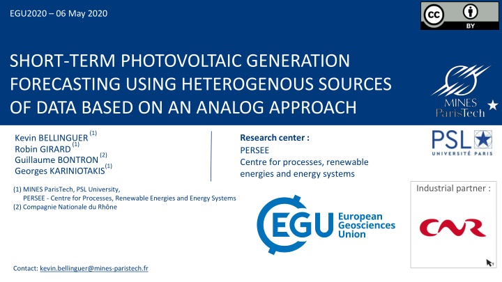
EGU2020 06 May 2020 SHORT-TERM PHOTOVOLTAIC GENERATION FORECASTING USING HETEROGENOUS SOURCES OF DATA BASED ON AN ANALOG APPROACH (1) Research center : PERSEE Centre for processes, renewable energies and energy systems Kevin BELLINGUER Robin GIRARD Guillaume BONTRON (1) (2) (1) Georges KARINIOTAKIS Industrial partner : (1) MINES ParisTech, PSL University, PERSEE - Centre for Processes, Renewable Energies and Energy Systems (2) Compagnie Nationale du Rh ne Contact: kevin.bellinguer@mines-paristech.fr
Plan I. II. Proposed approach I. A multi-inputs approach II. A conditioned learning III. Models definition / Case study IV. Outcomes and analysis V. Conclusions Objectives of PV forecasting 2
Objectives Proposed approach Models / Case study Outcomes Conclusion / Perspectives OBJECTIVES OF PV FORECASTING Weather dependence Production variability,limited controllability,uncertainties leads to large-scale integration problems New challenges to meet Management of the distribution network(balance, reserve, ) Optimization of maintenance scheduling Trading on electricity market What we propose: Short-term forecasting model (i.e. few minutes up to 6h ahead) A statistical approach A seamless model (i.e. a unique model suitable for large range of horizons) A simple model with good performances 3
Objectives Proposed approach Models / Case study Outcomes Conclusion / Perspectives A multi-inputs approach State of the art Classification of inputs used for PV production forecasting. Adapted from (Antonanzas, 2016) and (Diagne 2013). Photo credits: (M t o-France, meteociel.fr, (Ca adillas, 2018), CNR) State-of-the-art Production measurements Numerical Weather Prediction (NWP) Satellite images Sky images Inputs complementarity Due to their temporal & spatial resolutions, each approach observes specific phenomena NWP Satellite image Inputs combination Improvement of forecasting performance for short-term horizons (Aguiar 2016, Vallence 2018) Sky image Production measurements 4
Objectives Proposed approach Models / Case study Outcomes Conclusion / Perspectives The Spatio-Temporal approach Description Exploits the spatial and temporal correlations between the production data of spatially distributed PV sites Idea: a set of neighbouring PV plants is affected by the same clouds Short-term horizons (Bessa 2015) Spatio-Temporal approach Interests Data easily available (provided real time data logging) Improve forecasting performance up to 10% (Bessa 2015, Agoua 2018) Limitations PV sites spatial distribution (low density) Qualityof time series (converter shutdown, ) 5
Objectives Proposed approach Models / Case study Outcomes Conclusion / Perspectives A need for adaptivity Weather variability Variability in cloud cover leads to variability in PV production Models need to operate on a wide range of weather conditions (from sunny to overcast skies) An adaptative model is more accurate than a static model (Bacher, 2009) Proposed approach Hypothesis: similar PV production dynamics are observed under similar weather conditions Thus, fitting a model on all past PV observations can drown relevant information It seems wise to sample the learning set to obtain a weather coherent PV production observations subset in regard with the future weather state To do so, an analogy based approach is implemented 6
Objectives Proposed approach Models / Case study Outcomes Conclusion / Perspectives A conditioned learning An analog based approach: Past Construction of 2 past records for the same period Meteorological archive Observed PV production archive meteorological archive Retrieve forecast of analog predictors at time ? + ? Past observed PV production archive Compute the analogy score between the target meteorological situation and all the candidate situations from the meteorological archive. Each meteorological situation is ordered from the most similar to the less one. ? best meteorological situations are selected. Time Historical dataset ? ? + Legend The ? associated PV production observations are selected to train the forecasting model. Target meteorological situation Analogous meteorological situation Forecast of PV production at time ? + ?. Target PV production to forecast PV production observation used to fit models Which leads to an adaptative learning 7
Objectives Proposed approach Models / Case study Outcomes Conclusion / Perspectives An analog based approach Geopotential height fields Analog variable Geopotential field is chosen as an analog predictor Geopotential field is considered as a wind driver Analog metric Need to take into account the predictor spatial distribution Score S1 is used to measure similarity between the target and the candidate situations (Teweless and Wobus 1954, Obled, 2002) ?,?????? ?,? ? ?,?????????+ ? 1 ?=1 ?=1 ?,? ?,?????? ?,? ?,????????? ? 1 ?,? ? ?=1 ?=1 ?1= 100 Data integration Perfect prognosis mode Regarding target situation, reanalysis data are used instead of predictions Quantify the interest of using geopotential field as an analog predictor ?,??????, ?,? ? ?,????????? ? 1 ?=1 ?=1 max ?,? + ?,??????, ?,? ?,????????? ? 1max ? ?=1 ?=1 ?,? Terms are defined in the annex section 8
Objectives Proposed approach Models / Case study Outcomes Conclusion / Perspectives Data Stationarization Inputs stationarity ARIMA process requirement Get time series more easily forecastable Taken into account by stationarity procedure PV production variability Deterministic component: sun s path Stochastic component: clouds, aerosol, ????(?) ?????? ???(?) ?????? = Normalization Methods Clear-sky normalization (Bacher, 2009), (Agoua,2018) Seasonal decomposition (Cleveland, 1990), (Yang, 2012) Clear sky model used: McClear model (Lef vre, 2013) 9
Objectives Proposed approach Models / Case study Outcomes Conclusion / Perspectives Models definition Performance evaluation Score Skill Score ? ?????????( ) ?????????????( ) 1 ? ?=1 2 ?? = 1 ?? ?? ???? = Reference model: smart persistence ? 0 (?.?. ???????) ?= 0 (?.?. ??? ?????) ? ?? ?? ?? ?? ?? ? ??+ |? ? = ??+ 24? Auto-Regressive (AR) model ? ??+ |? = ? ? ? 0+ ? ?? ? ? ?=0 Terms are defined in the annex section 10
Objectives Proposed approach Models / Case study Outcomes Conclusion / Perspectives Conditioned learning A two steps conditioned learning approach (CAR model) First, the learning set is sample according to the hour of the day (CAR-T) Then, the previous subset is sample again in respect to the synoptic situations using the analogy based method (CAR-T.An) CARST-T.An + eXogenous inputs (CARXST) Conditioned Auto-Regressive (CAR-T.An) CAR-T.An + Spatio-Temporal data (CARST-T.An) ? ?,????+ ?? ? ? ? + ? ??+ |??+ + ? ?=0 ? ? ? ??????+ ????+ ? = ? ? ? ????+ ?? ? 0+ ? ?=0 ??, ??????+ ????? + ?=1 + nearby sites observations + satellite images On-site observations + NWP Terms are defined in the annex section 11
Objectives Proposed approach Models / Case study Outcomes Conclusion / Perspectives Features selection Least Absolute Shrinkage and Selection Operator (LASSO) To provide a seamless model, variable selection is carried out on each horizon to keep most informative features ?????=?????? 1 2??? ? + ? ? ? ? Location of the 10 most informative pixels Satellite pixels selection Rh ne valley topography To avoid a too large number of variables, we limits our approach to the 10 most informative pixels To quantify the correlation between the stationarized PV production and the stationarized satellite data for various lags, the Mutual Information Criterion is used (Carriere, 2020). The correlation area is highly influenced by the Rh ne valley topography. The shorter the horizon, the closer the most relevant pixels. For horizon higher than 3H00 ahead, most informative points are located westward. In this region, main wind seams to be westerly wind (see annex) 12
Objectives Proposed approach Models / Case study Outcomes Conclusion / Perspectives Case study Production measurements 9 PV plants D [7.3 ;133] km Pt= t =15 Pt Pnom, with ???? [1.2 ;12] ??p Satellite images Helioclim-3 (Blanc, 2011) Stationarized GHI t =15 NWP (exogenous inputs) ARPEGE M t o France Operational forecasting conditions Dissemination schedule Stationarized GHI t = 1H interpolated to t =15 ERA5 ECMWF Reanalysis Perfect prognosis mode Geopotential field at 500 & 925hPa t = 1H Analog predictor Wh/m Terms are defined in the annex section 13
Objectives Proposed approach Models / Case study Outcomes Conclusion / Perspectives Sensibility analysis Grid domains Parameters of the sensibility analysis Grid domains of the analog spatial window 3 regions centered over the Rh ne valley region Number of analogs situations to train the models From 50 up to 300 analogs situations Conclusions Grid domains The larger spatial window exhibits better performances. Number of analogs For very short-term horizons (i.e. from 15 up to 1H ahead), the more analogs, the better the performances, For longer horizons (i.e. from 2H up to 6H ahead), better performances are achieved with less analogous situations. 100 analog situations seems a good compromise. 14
Objectives Proposed approach Models / Case study Outcomes Conclusion / Perspectives Influence of the conditioned approach over performances Conclusions AR model Performance evaluation of the proposed conditioning approach over the reference model AR model outperforms the persistence up to ~15% for a 6H horizon. CAR-T model Conditioning of the learning set to the hour of day, improves performances in comparison with the AR model This phenomenon can be explained by: o The stationnarisation procedure is not perfect, especially for dawn times (Agoua, 2018) o The PV production dynamics varies according to the time of the day CAR-T.An The CAR-T.An model outperforms both the previous models. Compared to persistence model, improvement can reach ~24% for a 6H lead time Better performances are obtained when forecast model depends on the weather situation Model names are defined in the annex section 15
Objectives Proposed approach Models / Case study Outcomes Conclusion / Perspectives Comparison with a more advanced model Performance evaluation of the proposed conditioning approach with the Random Forest model (RF) Conclusions AR model The RF approach outperforms the AR model regardless of the considered forecasting horizon CAR model The proposed conditioning approach outperforms the RF and CRF models. Bad performances from CRF for very short times are supposed to result from over fitting Model names are defined in the annex section 16
Objectives Proposed approach Models / Case study Outcomes Conclusion / Perspectives Spatio temporal inputs CARST model Performance evaluation of the CAR model with ST inputs Conclusions CARST-T.An Model ST inputs (i.e. distributed sites and satellite pixels) improves performances for horizons below 6H00 ahead. Improvementare higher for 30 horizon and decrease with time At 6H00 horizon, the influence of ST is neglectable Model names are defined in the annex section 17
Objectives Proposed approach Models / Case study Outcomes Conclusion / Perspectives NWP inputs CARXST model Performance evaluation of the proposed models Conclusions CARST-T.An Model For horizon ranging from 15 up to 45 , performances improvement result from ST data CARXST-T.An Model From 1H up to 6H ahead horizon, the main source of performance improvement is due to NWP. Model names are defined in the annex section Seamless way to integrate capacity of NWP outputs to extend forecasting horizon 18
Objectives Proposed approach Models / Case study Outcomes Conclusion / Perspectives Conclusion et perspectives Conclusion The proposed conditioned learning improve performances up to 25% in comparison with a persistence model for a 6H ahead horizon ST data improve performances for horizon below 6H ahead, By ~4% for a 30 min horizon Improvement decrease progressively to become neglectable for a 6H horizon Combining the proposed conditioning approach with ST and NWP inputs, performances reach ~35% for a 6H lead time in regards with the persistence model The LASSO features selection enable to propose a seamless approach Perspectives Operational framework: consider NWP of geopotential fields rather than reanalysis Improve ST data integration by considering Cloud Motion Vector (CMV) approach 19
Objectives Proposed approach Models / Case study Outcomes Conclusion / Perspectives Thanks for your attention. 20
Objectives Proposed approach Models / Case study Outcomes Conclusion / Perspectives 21
Reference CHOWDHURY, RAHMAN, Forecasting sub-hourly solar irradiance for prediction of photovoltaic output, IEEE Photovoltaic Specialists Conference, 1987 CLEVELAND, CLEVELAND, MCRAE, STL - A seasonal-Trend Decomposition Procedure Based on Loess, Journal of Official Statistics , 1990 BACHER, MADSEN, NIELSEN, Online short-term solar power forecasting, Solar Energy, 2009 LORENZ, HURKA, HEINEMANN, Irradiance Forecasting for the Power Prediction of Grid-Connected Photovoltaic Systems, IEEE Journal of Selected Topics in Applied Earth Observations and Remote Sensing, 2009 YANG, JIRUTITIJAROEN, WALSH, Hourly solar irradiance time series forecasting using cloud cover index, Solar Energy, 2012 DIAGNE, DAVID, LAURET, Review of solar irradiance forecasting methods and a proposition for small-scale insular grids, Renewable and Sustainable Energy Reviews , 2013 DONG, YANG, REINDL, Short-term solar irradiance forecasting using exponential smoothing state space model, Energy, 2013 HUANG, KOROLKIEWICZ, AGRAWAL, Forecasting solar radiation on an hourly time scale using a Coupled AutoRegressive and Dynamical System (CARDS) model, Solar Energy, 2013 AKYUREK, KLEISSL, ROSING, TESLA - Taylor expanded solar analog forecasting, 2014 IEEE International Conference on Smart Grid Communications (SmartGridComm), 2014 ALESSANDRINI, DELLE MONACHE, SPERATI, An analog ensemble for short-term probabilistic solar power forecast, Applied Energy, 2015 BESSA, TRINDADE, MIRANDA, Spatial-Temporal Solar Power Forecasting for Smart Grids, IEEE Transactions on Industrial Informatics, 2015 ANTONANZAS, OSORIO, ESCOBAR, Review of photovoltaic power forecasting, Solar Energy, 2016 AGUIAR, PEREIRA, LAURET Combining solar irradiance measurements, satellite-derived data and a numerical weather prediction model to improve intra-day solar forecasting, Renewable Energy, 2016 GRADITI, FERLITO, ADINOLFI, Comparison of Photovoltaic plant power production prediction methods using a large measured dataset, Renewable Energy, 2016 AGOUA, GIRARD, KARINIOTAKIS, Short-Term Spatio-Temporal Forecasting of Photovoltaic Power Production, IEEE Transactions on Sustainable Energy, 2018 KAPOURCHALI, SPEHRY, ARAVINTHAN, Multivariate Spatio-temporal Solar Generation Forecasting: A Unified Approach to Deal With Communication Failure and Invisible Sites, IEEE Systems Journal, 2018 CANADILLAS, GONZALEZ-DIAS, RODRIGUEZ, A low-cost two-camera sky-imager ground-based intra-hour solar forecasting system with cloud base height estimation capabilities working in a smart grid, 2018 IEEE 7th World Conference on Photovoltaic Energy Conversion (WCPEC) , 2018 VAN DER MEER, WIDEN, MUNKHAMMAR, Review on probabilistic forecasting of photovoltaic power production and electricity consumption, Renewable and Sustainable Energy Reviews, 2018 CARRIERE, VERNAY, PITAVAL, KARINIOTAKIS, A Novel Approach for Seamless Probabilistic Photovoltaic Power Forecasting Covering Multiple Time Frames, IEEE Transactions on Smart Grid,pp. 1 1, 2019, BLANC, GSCHWIND, LEFEVRE, and WALD, The HelioClimProject: Surface Solar Irradiance Data for Climate Applications, Remote Sensing, vol. 3, no. 2, pp. 343 361, Feb. 2011 N. N. W. Service, Glossary - NOAA s National Weather Service, 00000 Library Catalog: w1.weather.gov. [Online]. Available: https://w1.weather.gov/glossary/index.php?letter=h OBLED, BONTRON, GARCON, Quantitative precipitation forecasts: a statistical adaptation of model outputs through ananalogues sorting approach, Atmospheric Research, vol. 63, no.3-4, pp. 303 324, Aug. 2002. 22
Glossary Abbreviation Definition Auto Regressive AR Auto Regressive model with Conditioned learning CAR Conditioned Auto Regressive model with Spatio-Temporal inputs CARST Conditioned Auto Regressive model with Spatio-Temporal and eXogenous inputs CARXST Cloud Motion Vector CMV Compagnie Nationale du Rh ne CNR Global Horizon Irradiance GHI Least Absolute Shrinkage and Selection Operator LASSO Numerical Weather Predictions NWP PhotoVoltaic PV Spatio Temporal ST Skill Score SS Random Forest RF 23
Model name definition Abbreviation Definition Auto Regressive model considering all available PV production observations AR Random Forest model considering all available PV production observations RF Auto Regressive model with Conditioned learning CAR AR model Conditioned to the Time of the day CAR-T AR model conditioned to the Time of the day and the synoptic state through an Analog based method CAR-T.An RF model conditioned to the Time of the day and the synoptic state through an Analog based method CRF-T.An Conditioned Auto Regressive model with Spatio-Temporal inputs CARST-T.An Conditioned Auto Regressive model with Spatio-Temporal and eXogenous inputs CARXST-T.An 24
S1 score Definition of the S1 score ?,?????? ?,? ?,?????? ?,? ?,????????? ? ? 1 ?,? ?,?????????+ ?=1 ? 1 ?=1 ? ?=1 ?=1 ?,? ?1= 100 ?,??????, ?,? ?,??????, ?,? ?,????????? ? ? 1max ?,????????? ? 1 ?=1 ? ?=1 + ?=1 ?=1 max ?,? ?,? ?,?= ??+1,? ? ? ?,? ?,?= ??,?+1 ??,? ? {??????,?????????} ? ? ?,? ??,? Where: ? The east-west geopotential gradient The north-south geopotential gradient ?,? ?,? ??,? The geopotential field at grid node (i,j) ? 25
Models parameters definition Parameters definition ??? Observed stationarized PV production at time t for plant x ??+ Predicted stationarized PV production at time t+h for plant x ??+ Synoptic weather situation expected at time t+h ???+ Conditioning approach based on synoptic situation and time of the day ? Regression coefficients ? Maximum lag of PV production observations (here, 2H) ? Neighbouring sites (here, 5 closest sites are considered) ???? ????+ StationarizedGHI forecast obtained from NWP output at plant x and time t+h ? ? Stationarized GHI observed at pixel i and time t ? Skill score definition ????????? ?????????????( ) ??????????? ????? ?? = ?????????????( ) =0 26
Main wind in the Rhne valley Principal Component Analysis (PCA) PCA is performed on 1 years of hourly reanalysis (ERA 5) of wind velocity at 750hPa The first Principal Component (PC) is represented at the opposite graph Westerly wind are observed 27