Signal Processing Fundamentals: Building Blocks and Basic Functions

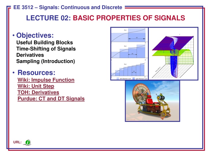
ECE 8443 Pattern Recognition EE 3512 Signals: Continuous and Discrete LECTURE 02: BASIC PROPERTIES OF SIGNALS Objectives: Useful Building Blocks Time-Shifting of Signals Derivatives Sampling (Introduction) Resources: Wiki: Impulse Function Wiki: Unit Step TOH: Derivatives Purdue: CT and DT Signals URL:

Introduction An important concept in signal processing is the representation of signals using fundamental building blocks such as sinewaves (e.g., Fourier series) and impulse functions (e.g., sampling theory). Such representations allow us to gain insight into the complexity of a signal or approximate a signal with a lower fidelity version of itself (e.g., progressively scanned jpeg encoding of images). In today s lecture we will investigate some simple signals that can be used as these building blocks. We will also discuss some basic properties of signals such as time-shifting and basic operations such as integration and differentiation. We will learn how to represent continuous-time (CT) signals as a discrete-time (DT) signal by sampling the CT signal. EE 3512: Lecture 02, Slide 1

The Impulse Function The unit impulse, also known as a Delta function or a Dirac distribution, is defined by: ( ) 0 , 0 = t t 1/ / 2 ( ) d = , 1 for any real number 0 / 2 The impulse function can be approximated by a rectangular pulse with amplitude A and time duration 1/A. t K For any real number, K: / 2 / 2 ( ) ( ) d = d = , for 0 K K K / 2 / 2 t This is depicted to the right. The definition of an impulse for a DT signal is: = = 0 , 0 n . 1 = = n x.JPG , 1 0 n [ ] n n Note that: EE 3512: Lecture 02, Slide 2

The Unit Step and Unit Ramp Functions We can define a unit step function as the integral of the unit impulse function: x.JPG t ( ) t = = ( ) , 0 for 0 u t d t t ( ) ( ) = = = , 1 for 0 d d t t This can be written compactly as: = 0 , 0 t x.JPG , 1 0 t ( ) t u Similarly, the derivative of a unit step function is a unit impulse function. t We can define a unit ramp function as the integral of a unit step function: xx.JPG t ( ) t = = ( ) , 0 for 0 r t u d t t ( ) ( ) = = = , for 0 u d u d t t 0 EE 3512: Lecture 02, Slide 3

The DT Unit Step and Unit Ramp Functions xx.JPG We can sum a DT unit pulse to arrive at a DT unit step function: n m = m = = [ ] , 0 for 0 u n n n n m 0 m = m = m = = + = + = 1 0 , 1 for 0 n 1 x.JPG We can define a time-limited pulse, often referred to as a discrete-time rectangular pulse: = , 1 ( / ) 1 ,..., 2 1 , 0 , 1 ,..., ( / ) 1 2 n L L = [ ] pL n , 0 all other n x.JPG We can sum a unit step to arrive at the unit ramp function: n n m = m = = , 0 for 0 r u n n n m m = m = m = = = , for 0 u n n 0 EE 3512: Lecture 02, Slide 4

Sinewaves and Periodicity Sine and cosine functions are of fundamental importance in signal processing. Recall: ( ) j t e cos + = x.JPG ( ) t j t sin A sinusoid is an example of a periodic signal: = + ( ) cos( ), x t A t t A sinusoid is period with a period of T = 2 / : 2 ( cos( + + = + + = + ) ) cos( 2 ) cos( ) A t A t A t Later we will classify a sinewave as a deterministic signal because its values for all time are completely determined by its amplitude, A, is frequency, , and its phase, . Later, we will also decompose signals into sums of sins and cosines using a trigonometric form of the Fourier series. EE 3512: Lecture 02, Slide 5

Time-Shifted Signals Given a CT signal, x(t), a time-shifted version of itself can be constructed: x(t-t1) delays the signal (shifts it forward, or to the right, in time), and x(t+t1), which advances the signal (shifts it to the left). x.JPG We can define the sifting property of a time-shifted unit impulse: + t t 1 ( ) ( ) = ( ), for any 0 f t d f t 1 1 1 ( ) ( ) ( ) ( 1 t ) = We can easily prove this by noting: f t f t 1 1 and: + + + t t t 1 1 1 ( ) ( ) ( ) ( 1 t ) ( ) 1 t ( ) 1 t 1 t 1 t d = d = d = = ( ) ) 1 ( ( ) f t f t f t f t f t 1 1 1 1 1 EE 3512: Lecture 02, Slide 6

Continuous and Piecewise-Continuous Signals A continuous-time signal, x(t), is discontinuous at a fixed point, t1, if where are infinitesimal positive numbers. 1 1 t x t x 1 1 1 1 and t t t t ( ) ( ) + + ( ) 1 t ( ) 1 t ( ) 1 t + = = x x x 1t A signal is continuous at the point if . If a signal is continuous for all points t, x(t) is said to be a continuous signal. Note that we use continuous two ways: continuous-time signal and continuous (as a function of t). x.JPG The ramp function, r(t), and the sinusoid are examples of continuous signals, as is the triangular pulse shown to the right. A signal is said to be piecewise continuous if it is continuous at all t except at a finite or countably infinite collection of points ti,i = 1, 2, 3, x.JPG EE 3512: Lecture 02, Slide 7

Derivative of a Continuous-Time Signal ( ) t 1 + ( ) x t h x 1 A CT signal, x(t), is said to be differentiable at a fixed point, t1, if has a limit as h 0: t dx ) ( = = h ( ) t 1 + ( ) x t h x 1 lim dt h 0 h t t 1 independent of whether h approaches zero from h> 0 or h< 0. To be differentiable at a point t1, it is necessary but not sufficient that the signal be continuous at t1. Piecewise continuous signals are not differentiable at all points, but can have a derivative in the generalized sense: ( ( ) 1 t ( ) 1 t ( ) dx t ) + + x x t t 1 dt ( ) t is the ordinary derivative of x(t) at all t, except at t= t1. is an impulse concentrated a t= t1 whose area is equal to the amount the function jumps at the point t1. dx ) ( t dt x.JPG For example, for the unit step function, the generalized derivative of is: ( ) t u u K 0 0 ( ) t Ku ( ( ) ) ( ) t + = 0 K EE 3512: Lecture 02, Slide 8

DT Signals: Sampling One of the most common ways in which discrete-time signals arise is sampling of a continuous-time signal. In this case, the samples are spaced uniformly at time intervals where T is the sampling interval, and 1/T is the sample frequency. Samples can be spaced uniformly, as shown to the right, or nonuniformly. x.JPG tn= nT We can write this conveniently as: ) ( x t x n x nT t = = = xx.JPG ( ) nT Later in the course we will introduce the Sampling Theorem that defines the conditions under which a CT signal can be recovered EXACTLY from its DT representation with no loss of information. Some signals, particularly computer generated ones, exist purely as DT signals. EE 3512: Lecture 02, Slide 9

Summary Representation of signals using fundamental building blocks can be a useful abstraction. We introduced four very important basic signals: impulse, unit step, ramp and a sinewave. Further we introduced CT and DT versions of these. We introduced a mathematical representation for time-shifting a signal, and introduced the sifting property. We discussed the concept of a continuous signal and noted that many of our useful building blocks are discontinuous at some point in time (e.g., impulse function). Further DT signals are inherently discontinuous. We introduced the concept of a derivative of a continuous signal and noted that the derivative of a discrete-time signal is a bit more complicated. Finally, we presented some introductory material on sampling. EE 3512: Lecture 02, Slide 10