Learn how to use Simple Regression Analysis to evaluate the impact of a single input variable on a continuous output variable. Explore regression models, interpretation of coefficients, and significance levels through practical examples and graphical outputs. Enhance your data analysis skills with this powerful statistical tool.
Please find below an Image/Link to download the presentation.
The content on the website is provided AS IS for your information and personal use only. It may not be sold, licensed, or shared on other websites without obtaining consent from the author. If you encounter any issues during the download, it is possible that the publisher has removed the file from their server.
You are allowed to download the files provided on this website for personal or commercial use, subject to the condition that they are used lawfully. All files are the property of their respective owners.
The content on the website is provided AS IS for your information and personal use only. It may not be sold, licensed, or shared on other websites without obtaining consent from the author.
E N D
Presentation Transcript
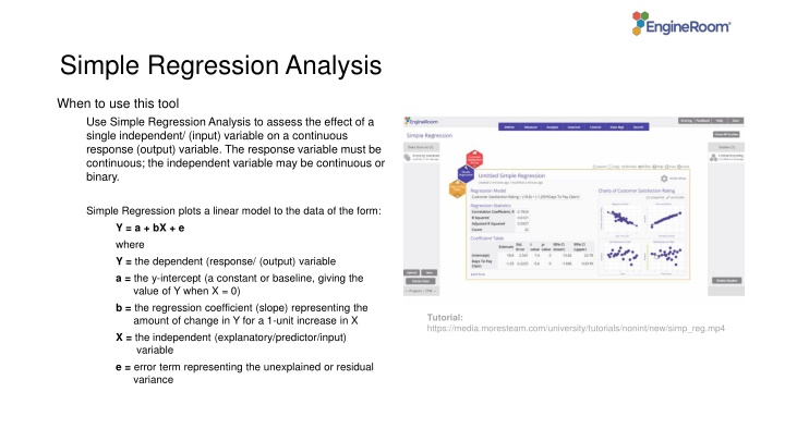
Simple Regression Analysis When to use this tool Use Simple Regression Analysis to assess the effect of a single independent/ (input) variable on a continuous response (output) variable. The response variable must be continuous; the independent variable may be continuous or binary. Simple Regression plots a linear model to the data of the form: Y = a + bX + e where Y = the dependent (response/ (output) variable a = the y-intercept (a constant or baseline, giving the value of Y when X = 0) b = the regression coefficient (slope) representing the amount of change in Y for a 1-unit increase in X X = the independent (explanatory/predictor/input) variable e = error term representing the unexplained or residual variance Tutorial: https://media.moresteam.com/university/tutorials/nonint/new/simp_reg.mp4 Tutorial: https://media.moresteam.com/university/tutorials/nonint/new/simp_reg.mp4
Using EngineRoom Analyze > Regression Analysis > Simple Regression
Using EngineRoom There are two 'drop zones' attached to the study: Response Variable (required): for the variable containing the output measurements. Must be numeric (and is assumed continuous). Independent Variable (required): for the variable containing the input levels or measurements. Can be numeric or text.
Simple Regression Example simplereg_exmpldata.xlsx simplereg_exmpldata.xlsx Steps: The example dataset contains data collected over 22 days on an output variable (Y), Customer Satisfaction Rating, and an input variable (X), Days to Pay Claim, along with the observation numbers (Data Pair). Click on the data file in the data sources panel and drag Days to Pay Claim onto the Independent Variable drop zone. Drag Customer Satisfaction Rating onto the Response Variable drop zone. Enter the value of the desired risk or significance level (this should be a value between 0 and 1, conventionally 0.05 or 0.1) or leave the default value of 0.05 as is. Click Continue We will analyze these data to see whether Days to Pay Claim (X) accounts for the bulk of the variation in Customer Satisfaction (Y).
Simple Regression Example Output The model is significant (p-value = 0) and explains over 60% of the variation in Customer satisfaction (R-squared = 0.61)
Simple Regression Example Output The graphical output contains: Scatter plot of the input (X = Days to Pay Claim) vs. output (Y = Customer Satisfaction Rating) showing the line of best fit. And three residual plots: Normal Q-Q (quantile- quantile) plot which is like a probability plot. If the plotted points fall along the diagonal line, the assumption that residuals are normally distributed, holds. Scatter plot of Standardized residuals vs. the time order of the observations. If the plotted points are randomly scattered with no patterns or trends, the assumption of independent residuals holds. Scatter plot of Standardized residuals vs. fitted values (predictions of the data observations using the regression model). If the plotted points are randomly scattered with no patterns or trends, the assumption of independent residuals holds.
Simple Regression Example Output The numeric output contains: Regression model expressed as a line equation Regression statistics table showing the correlation coefficient (r ), coefficient of determination (R- square = R^2), Adjusted R-square (adjusted for the total number of X variables in the model) and the count (sample size) Coefficient Table ANOVA Table