Simulating Uncertainty Lecture 16
In this lecture, the difference between risk and uncertainty is explored, emphasizing the role of known versus unknown probability distributions. The concept of hybrid distributions and modeling low probability, high impact events are discussed, shedding light on the importance of considering subjective risk augmentation. The GRKS distribution for cases with limited historical data is also touched upon, providing insights into handling uncertainties effectively.

Download Presentation

Please find below an Image/Link to download the presentation.
The content on the website is provided AS IS for your information and personal use only. It may not be sold, licensed, or shared on other websites without obtaining consent from the author.If you encounter any issues during the download, it is possible that the publisher has removed the file from their server.
You are allowed to download the files provided on this website for personal or commercial use, subject to the condition that they are used lawfully. All files are the property of their respective owners.
The content on the website is provided AS IS for your information and personal use only. It may not be sold, licensed, or shared on other websites without obtaining consent from the author.
E N D
Presentation Transcript
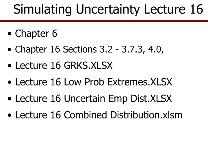
Simulating Uncertainty Lecture 16 Chapter 6 Chapter 16 Sections 3.2 - 3.7.3, 4.0, Lecture 16 GRKS.XLSX Lecture 16 Low Prob Extremes.XLSX Lecture 16 Uncertain Emp Dist.XLSX Lecture 16 Combined Distribution.xlsm
Risk vs. Uncertainty Risk is when we have random variability from a known (or certain) probability distribution Uncertainty is when we have random variability from unknown (or uncertain ) distributions Known distribution can be a parametric or non-parametric distribution Normal, Empirical, Beta, etc.
Uncertainty We have random variables coming from unknown or uncertain distributions May be based on history or on purely random events or reactions by people in the market place Could be a hybrid distribution as Part Normal and part Empirical Part Beta and part Gamma We are uncertain and must test alternative Dist.
Uncertainty Conceptualize a hybrid distribution Part Normal and part Empirical Simulate a USD as USD = uniform(0,1) If USD <0.2 then = * (1+EMP(Si, F(x))) IF USD>=0.2 and USD<=0.8 then = NORM( , Std Dev) If USD > 0.8 then = * (1+EMP(S i, F (x))) Where S iare sorted large values for Y and Si are sorted small values for Y
Uncertainty This is how we will model low probability, high impact events, i.e., Black Swans The event may have a 1 or 2% chance but it would mean havoc for your business Low risk events must be included in the business model or you will under estimate the potential risk for the business decision This is a subjective risk augmentation to the historical distribution
GRKS Distribution for Uncertainty When you have little or no historical data for a random variable assume a distribution such as: GRKS (Gray, Richardson, Klose, and Schumann) Or EMP I prefer GRKS because Triangle never returns min or max and we usually ask manager for the min and max that is observed 1 in 10 years, i.e., a 10% chance of occurring
GRKS Distribution GRKS parameters are Min, Middle or Mode, and Max Define Min as the value where you have a 97.5% chance of seeing greater values Define Max as the value where there is a 97.5% chance of seeing lower values In other words, we are bracketing the distribution with 2 standard deviations GRKS has a 50% chance of seeing values less than the middle Once estimated the parameters can be adjusted
GRKS Distribution 1.0 min middle max min middle max Parameters for GRKS are Min, Middle, Max Simulate it as =GRKS(Min, Middle, Max) Note: not necessarily equal distance from middle =GRKS(12, 20, 50)
GRKS Distribution Easy to modify the GRKS distribution to represent any subjective risk or random variable. This makes the dist. very flexible From the Simetar Toolbar click on GRKS Distribution and fill in the menu Edit table of deviates for Xs and F(Xs) to change the distribution shape to conform to your subjective expectations Simulate distribution using =EMP(Si , F(x))
GRKS Distribution The GRKS menu asks for Minimum Middle Maximum No. of intervals in Std Deviations beyond the min and max. I like 4 intervals to give more flexibility to customizing the distribution. Always request a chart so you can see what your distribution looks like after you make changes in the X s or Prob(x) s
Modeling Uncertainty with GRKS The GRKS menu generates the following table and CDF chart: Prob(Xi) is the Y axis and Xi is the X axis Has 13 equal distant intervals for X s; so we have parameters for EMP 50% observations below Mode 2.275% below the Minimum 2.275% above the Maximum
Modeling Uncertainty with GRKS 3. If you want to modify the distribution, edit the values in the table. To demonstrate this I repeated Step 2 and then modified the Xi values in the table below. The assumption is that I think Y should be 50 about 35% of the time. The values in Prob(Xi) and Xi that I changed are in Bold. GRKS Distribution With the Following Parameters: Minimum Mode 25 Interval Prob(Xi) Pseudo Min 1 2 Minimum 3 4 5 6 Mode 7 8 9 10 Maximum 11 12 Pseudo Max 13 Maximum 65 100 GRKS Distribution Xi 0.00 0.01 0.02 0.07 0.16 0.35 0.50 0.69 0.84 0.93 0.98 0.99 1.00 0.00 50.00 50.00 50.00 50.00 50.00 65.00 73.75 82.50 91.25 100.00 108.75 117.50 1.00 0.90 0.80 0.70 0.60 0.50 0.40 0.30 0.20 0.10 0.00 40.00 50.00 60.00 70.00 80.00 90.00 100.00 110.00 120.00
Modeling Uncertainty with EMP Actually it is easy to model uncertainty with an EMP distribution We estimate the parameters for an EMP using the EMP Simetar icon for the historical data Select the option to estimate deviates as a percent of the mean or trend Next we modify the probabilities and Xs based on your expectations or knowledge about the risk in the system
Modeling Uncertainty with EMP Below is the input data and the EMP parameters as fractions of the trend forecasts Note price can fall a maximum of 25.96% from Price can be a max of 20.54% greater than
Modeling Uncertainty with EMP The changes I made are in Bold. Then calculated the Expected Min and Max. F(X) is used for all three random variables. You may not want to do this. You may want a different F(x) for each variable.
Modeling Uncertainty with EMP Results from simulating the modified distribution for Price Note probabilities of extreme prices
Modeling Uncertainty with EMP Comparison of CDFs for Original and Modified Price Distributions 1 0.9 0.8 0.7 0.6 Prob 0.5 0.4 0.3 0.2 0.1 0 3 5 7 9 11 13 15 Price 1 Price 2
Summary Modeling Uncertainty Do not assume historical data has all the possible risk that can affect your business Use yours or an expert s experience to incorporate extreme events which could adversely affect the business Modify the historical distribution based on expected probabilities of rare events See the next side for an example.
Modeling Low Probability Extremes Assume you buy an input and there is a small chance (2%) that price could be 150% greater than your Historical risk from EMP function showed the maximum increase over is 59% with a 1.73% I would make the changes to the right in bold and simulate the modified distribution as an =EMP() Simulation results are provided on the right