Simulink Basics: Getting Started with Simulations and Components
Explore the fundamentals of Simulink, a simulation tool in Matlab, including setting up simulations, using components like Scope block, calculus operations, transfer functions, and modeling digital circuits. Learn how to start Simulink, view waveforms, implement feedback, and more.

Download Presentation

Please find below an Image/Link to download the presentation.
The content on the website is provided AS IS for your information and personal use only. It may not be sold, licensed, or shared on other websites without obtaining consent from the author. If you encounter any issues during the download, it is possible that the publisher has removed the file from their server.
You are allowed to download the files provided on this website for personal or commercial use, subject to the condition that they are used lawfully. All files are the property of their respective owners.
The content on the website is provided AS IS for your information and personal use only. It may not be sold, licensed, or shared on other websites without obtaining consent from the author.
E N D
Presentation Transcript
Introduction to Matlab Module #9 Simulink Topics 1. Simulink Textbook Reading Assignments 1. 9.1-9.5 Practice Problems 1. 9.1, 9.3, 9.6, 9.31 Module #9 Page 1 Introduction to Matlab
1) Simulink Starting Simulink - type simulink at the prompt >> simulink - File New Model - Model files are saved as .mdl - The Simulink Library contains built in components that can drag-n-dropped in your library file Module #9 Page 2 Introduction to Matlab
1) Simulink Starting Simulink - Simulations can be setup using the pull-down menu: Simulation Configuration Settings - This is similar to a SPICE simulation where you specify start time, stop time, step size. Module #9 Page 3 Introduction to Matlab
1) Simulink Starting Simulink - The Scope block can be used to view the analog diagrams of signals within the block diagram. - Connections are made by clicking-and-holding on the block ports and dragging to the destination block OR by selecting the source block, holding the cntl-key, then clicking on the destination block - Parameters of each block can be set by double-clicking on the component - A simulation is ran by pressing the Play button Module #9 Page 4 Introduction to Matlab
1) Simulink Starting Simulink - after the simulation ends, you can double-click on the Scope block to see the waveform. Module #9 Page 5 Introduction to Matlab
1) Simulink Calculus Operations, Feedback, and Gain - The summing component is used for positive and negative feedback. - The polarity of the feedback is set in the List of Signs parameter by listing + s and s. - Calculus operations are entered using their Laplace Transform symbols Differentiation Integration = s = 1/s - Multiple signals can be viewed on the scope using the Bus Creator component Module #9 Page 6 Introduction to Matlab
1) Simulink Transfer Functions can be used to describe behavior. Module #9 Page 7 Introduction to Matlab
1) Simulink Digital Circuits Can Be Modeled Module #9 Page 8 Introduction to Matlab
1) Simulink Outputting to the Workspace - The Sinks/To Workspace block provides a way to send the output of Simulink to a variable in Matlab - When using the To Workspace block, you should change the variable name to something descriptive and change the Save Format as Array - The Signal Routing/Mux block provides a way to send multiple variables to the workspace - The Sources/Clock block provides a way to record the time. Module #9 Page 9 Introduction to Matlab
1) Simulink Plotting Solutions to Differential Equations - The solution to differential eqs can be plotted by building up the equation graphically. Ex) plot the solution to this equation from 0 < t < 6 dy 2 d y = ) 0 ( 1 = ) 0 ( y 4 where and = + 10 7 sin( 4 ) 5 cos( 3 ) t t dt 2 dt - first, we need to rearrange the expression so that it is in a form of y(t) = .. + 2 7 sin( 4 ) 5 cos( 3 ) d y t t = 2 10 dt + 10 2 7 sin( 4 ) 5 cos( 3 ) d y t t = 2 dt + 10 7 sin( 4 ) 5 cos( 3 ) t t = ( ) y t Module #9 Page 10 Introduction to Matlab
1) Simulink Plotting Solutions to Differential Equations + 10 7 sin( 4 ) 5 cos( 3 ) t t = ( ) y t - The cosine block is created using the sine block with a phase shift of pi/2 - The amplitudes and frequencies for the sine and cosine are entered within the source blocks - The initial condition y(0) = 4 is set in the Integrator1 block - The initial condition y (0) = 1 is set in the Integrator2 block Module #9 Page 11 Introduction to Matlab
1) Simulink Plotting Solutions to Linear Equations = y 3 4 5 x y ex) = 6 10 2 x - We can rearrange variables to get expressions in terms of x = x y 6 ( / ) 2 10 y x = / ) 5 3 ( 4 - We enter these expressions into simulink and produce output functions of a linear ramp of x (-10 to 10 in ramp and sim time) - The intersection of the lines represents the solution (x=7, y=4) Module #9 Page 12 Introduction to Matlab
1) Simulink Subsystems - repetitive functions can be put into subsystems with a unique symbol. - there are two methods to make subsystems 1) Dragging the Subsystem block from the library 2) Creating a block diagram first that contains portsand then encapsulating it and creating an automatic subsystem block of everything encapsulated. Ex) - Create a block diagram and insert input/output ports - Select everything, right-click, create subsystem Module #9 Page 13 Introduction to Matlab
1) Simulink Subsystems - The subsystem can be copied/pasted - The subsystem can be pushed into by double clicking on it - there are two methods to make subsystems 1) Dragging the Subsystem block from the library 2) Creating a block diagram first that contains portsand then encapsulating it and creating an automatic subsystem block of everything encapsulated. Ex) Module #9 Page 14 Introduction to Matlab

 Simulink")
 Simulink")
 Simulink")
 Simulink")
 Simulink")
 Simulink")
 Simulink")
 Simulink")
 Simulink")
 Simulink")
 Simulink")
 Simulink")
 Simulink")