Socialist Growth Revisited: Insights from Yugoslavia
This study delves into the economic performance of Yugoslavia, highlighting the shift from planned economies to decentralized systems and the impact on growth. By analyzing macroeconomic indicators and historical context, the research sheds light on the challenges and nuances of socialist growth strategies.

Download Presentation

Please find below an Image/Link to download the presentation.
The content on the website is provided AS IS for your information and personal use only. It may not be sold, licensed, or shared on other websites without obtaining consent from the author.If you encounter any issues during the download, it is possible that the publisher has removed the file from their server.
You are allowed to download the files provided on this website for personal or commercial use, subject to the condition that they are used lawfully. All files are the property of their respective owners.
The content on the website is provided AS IS for your information and personal use only. It may not be sold, licensed, or shared on other websites without obtaining consent from the author.
E N D
Presentation Transcript
Socialist Growth Revisited: Insights from Yugoslavia Leonard Kuki London School of Economics, Department of Economic History
Introduction (I) Successor states of Yugoslavia have essentially stagnated over the past 30 years. Diverging European economic development after WWII had attracted much public interest. Not academic interest necessarily. Planned economies performed relatively well in the 1950s and the 1960s. In the 1980s their performance turned dismal. (Usual) Explanation: Growth based on capital and labour expansion, and the transfer of resources from farms to factories, intrinsically limited (Krugman, 1995).
Introduction (II) Failure of planned economies mostly attributed to embedded inefficiencies. Doom argument: Employers and employees faced poor incentives since property was state owned (Bardhan and Roemer, 1993). Nuanced argument: performance was relatively OK during mass production 1950s/1960s. But bad with onset of flexible production technologies during late 1970s (Broadberry and Klein, 2011) . technology of the
Motivation (I) Existing literature suffers from two problems. 1stProblem: Excessive focus on Soviet Union. Masks heterogeneity of E. European countries. I analyse Yugoslavia. Yugoslavia was taken as an example of one of fastest growing countries in 1950-70s. Thus, Balassa and Bertrand (1970) found Yugoslavia did better than the average of other 9 sample countries, in terms of output and TFP growth. In AER, Horvat (1971) attributed this to Yugoslavia s decentralised economic system.
Motivation (III): The evolution of macroeconomic indicators in Yugoslavia and in the U.S., 1952-90. Figure 1.1: GDP per capita Figure 1.2: Capital to labour ratio 90 70 70 50 50 1990 Int. GK$, log scale 1990 Int. GK$, log scale 30 30 10 10 5 5 2 2 1952 1960 1970 Year 1980 1989 1952 1960 1970 Year 1980 1989 Figure 1.3: Investment to output ratio Figure 1.4: Hours worked per capita 0.5 0.7 0.4 0.6 Hours per person 0.3 0.5 Ratio 0.2 0.4 0.1 0.3 0 0.2 1952 1960 1970 Year 1980 1989 1952 1960 1970 Year 1980 1989 Yugoslavia U.S. Note: Capitais defined as working age person, while labour is defined as total hours worked ((average yearly hours worked per employee) x (total number of employees)). Hours worked per capita are total hours worked divided by the working age population.
Motivation (IV) 2nd Literature problem: Typically relies on a simple comparison of macro indicators, like productivity and growth (van Ark, 1996; Broadberry and Klein, 2011). Hence, arguments not quantified or tested. Some growth accounting exercises (Balassa and Bertrand, 1970; Vonyo, 2010). Very useful, but growth acc. suffers from its own problems. So what can be done?
Motivation (V) I apply business cycle accounting (BCA). Developed by Cole and Ohanian (2002) and Chari et al. (2007), among others. BCA is a diagnostic tool like growth accounting, but moves towards explanations. Hence, I can explain both the success and failure episodes. 1. 2. BCA composed of two steps: Calculate from data. Insert wedges into a prototype model to determine their impact on econ. growth. 1. 2. As a dynamic general equilibrium (DGE) model, confers two major advantages. Adds a timing dimension. Identifies the incentives that drive output, capital and labour.
Preview of results 1. TFP became more important over time in sustaining growth. Reconciles conflicting results in literature about relative importance of factors and TFP (Balassa and Bertrand, 1970; Weitzman, 1970; Sapir, 1980; Bergson, 1983; Kontorovich, 1986). 2. The labour wedge consistently deteriorated since the mid-1960s. And drove the collapse of growth during the 1980s. Similar to findings of Weitzman (1970), Sapir (1980), and Easterly and Fischer (1995). But on completely different grounds. Does not mean that technology and diminishing returns on capital were un-important. Rather, labour frictions were more important.
History Evolution of socialist economic system can be divided into four phases. Gradual move from central planning, through market socialism, to decentralised planning. 1st Phase, 1947-1951: Rigid central planning focused on heavy industrialisation. Soviet Union Template. 2nd Phase, until 1965; Yugoslav officials sought to distance themselves from Soviet Union. Yugoslavia began gradually opening towards the West. 3rd Phase, until 1975: 1965 reform important. Heyday of market socialism. Economic power further decentralised to work councils within firms. 4rd Phase, until the end: 1974 constitution led to further decentralisation of power to the level of departments within firms.
History IV: Trade as per cent of GDP (1990 Int. GK$), and composition of trade, 1952- 1988. 90 80 70 60 % 50 40 30 20 10 0 1952 1953 1954 1955 1956 1957 1958 1959 1960 1961 1962 1963 1964 1965 1966 1967 1968 1969 1970 1971 1972 1973 1974 1975 1976 1977 1978 1979 1980 1981 1982 1983 1984 1985 1986 1987 1988 Year Trade as % of GDP OECD as % of total trade Socialist Bloc as % of total trade Note: This measure of openness can be considered real, since GDP is PPP adjusted. Trade means exports and imports of goods and services. Composition of trade, however, reefers to composition of trade in goods, due to data constraints.
History V: Western aid as per cent of GDP and gross investments (1990 Int. GK$), 1952-1965. 12.00 10.00 8.00 6.00 % 4.00 2.00 0.00 1952 1953 1954 1955 1956 1957 1958 1959 1960 1961 1962 1963 1964 1965 Year % of gross investments % of GDP
Methodology BCA based on a standard Ramsay-Cass-Koopmans growth model. Chari et al. (2007) argue that a large set of DGE models can be simplified through addition of wedges . BCA developed for accounting for business cycle fluctuations. But can be applied to study episodes of economic growth (Lahiri and Yi, 2009; Lu, 2012; Chakraborty and Otsu, 2013; Cheremukhin et al., 2014.
Intuition (I) BCA cannot identify the policies that effect the economy, bur rather the evolution of incentives that firms and households face. Four wedges used are channels through which policies affect growth. Taken together, they drive economic growth, and match data. Labour wedge is related to incentives that determine the supply of labour. Increasing labour wedge can be interpreted as an increase in the return for work effort. Capital wedge is related to incentives that determine savings and investments, both physical and human capital. Increasing capital wedge can be interpreted as an increase return on capital.
Intuition (II) Income wedge embodies aggregate demand shocks stemming from G and NX. Efficiency wedge (TFP) measures the efficiency with which inputs are transformed into output. Drawbacks: 1. Wedges do not interact. 2. Can t identify the exact incentives.
Prototype model: Setup Utility f.: Budget constraint: Production function: Capital law of motion:
Equilibrium with wedges (I) Efficiency wedge: . As in RBC models, is measured as the deviation around (labour augmenting tech. progress). Labour wedge: . Measures discrepancy between and MPL.
Equilibrium with wedges (II) Capital wedge: (1+?)??+1 ??? + ? 1 = ???+1 1 ??,?+1. ??+1 Measures the discrepancy between intertemporal substitution and the real interest rate. Income wedge: ?? ?? ??= ????,?. Measures the expenditure gap for the resource constraint to hold.
Data (I) Official output series problematic (Social Product). Services excluded (education, healthcare, government, and etc.). But input from excluded services into other sectors included. Gross inconsistency in the application of the Material Planning System. 1. Index number problems (Gerschenkron, 1947). 2. Distorted prices (Staller, 1986). 3. Perhaps outright fabrication. Furthermore, official output growth inflated due to: As such, I use output series from Maddison (2010). But created by Thad Alton et al. (1970, 1992).
Data (II) Working age population (15-64), employment of social sector, and data on private farming employment taken from official sources. Total yearly labour input de-trended by 3600. Human capital initially approximated by average years of schooling from Barro and Lee (2013). I take their estimate for Serbia. Avg. years of schooling turned into mincerian human capital as in Hall and Jones (1999). Capital stock series problematic. Exclude an investment category called other .
Calibration Assume ? is 0.95, and assume that ? is 2, as in similar countries (Lu, 2012; Cheremukhin et al., 2014). ? is 0.4, as in Easterly and Fischer (1995). Kukic (2015) finds 0.43 for Yugoslavia. Remaining parameters taken from data. ?? is time-varying, and on average 1.1 % per annum. ? is 0.9 % (constant). ? is 5.46 %, to ensure modelled capital stock matches the 1990 data.
Assumptions 1990 is the terminal period of wedges. Profit maximisation is a poor description of socialist firms. But a socialist economy can be seen as a heavily distorted version of a perfectly competitive economy. Cobb-Douglas assumption of unit substitution between capital and labour is problematic (Weitzman, 1970; Sapir, 1980; Easterly and Fischer, 1995). Might be below one. If so, provides an elegant explanation for socialist growth - planned economies ran into acute diminishing returns on capital.
Results:The evolution and interpretation of wedges Figure 4.1: TFP Figure 4.2: Capital wedges 280 1.5 Frictionless benchmark model =1 Steady State in benchmark =100 260 240 220 200 1 180 160 0.5 140 120 100 0 1952 1960 1970 Year 1980 1989 1952 1960 1970 Year 1980 1989 Figure 4.3: Labor wedges Figure 4.4: Income wedges (as a share of GDP) 1.6 0.5 Frictionless benchmark model =1 Percentage of output (Y) 1.4 0.4 1.2 1 0.3 0.8 0.2 0.6 0.4 0.1 1952 1960 1970 Year 1980 1989 1952 1960 1970 Year 1980 1989 Yugoslavia U.S. Note: Business cycles have been cycled out using the Hodrick-Prescott filter (smoothing parameter = 6.25). No technological growth rate is imposed ( = 0), rendering TFP growth comparable to standard growth accounting exercises.
Interpreting TFP (I) Nishimizu and Page (1982) argue that TFP was driven by efficiency rather than technology. Similar to Hsieh and Klenow (2009). Viable interpretations: 1. Reconstruction dynamics (Vonyo, 2008). 2. Structural change or improvements in sectoral allocation of resources (Lewis, 1954; Vollrath, 2009).
Interpreting TFP (II): Share of agricultural workers in total workforce in Yugoslavia, 1952-89 0.8 0.7 0.6 0.5 Share 0.4 0.3 0.2 0.1 0 1952 1953 1954 1955 1956 1957 1958 1959 1960 1961 1962 1963 1964 1965 1966 1967 1968 1969 1970 1971 1972 1973 1974 1975 1976 1977 1978 1979 1980 1981 1982 1983 1984 1985 1986 1987 1988 1989 Year
Interpreting TFP (III) Trade might had boosted output through TFP (Alcala and Ciccone, 2004). Yugoslavia did specialise according to its comparative advantage.
Interpreting labour wedge (I) Hall (1997) argues labour wedge reflects frictions that lead households to spend a long time on non-market activities. Figure 6.1: Total hours worked 18 17 In billions 16 15 14 1952 1960 1970 Year 1980 1989 Figure 6.2: Working age population 17 16 15 In millions 14 13 12 11 10 1952 1960 1970 Year 1980 1989
Interpreting labour wedge (II) Mismatch between total hours worked and the working age population reflected in increasing unemployment. Unemployment rate an average 8.2 per cent during 1967-75, rose to an average 12.6 percent during 1976-87. Migration patterns not helpful.
Interpreting labour wedge (III) Chari et al. (2007) argue that labour wedge can reflect distortions caused contraction (deflation) and trade unions (nominal wage rigidity). by monetary In Yugoslavia during 1980s, real money balances halved (Bradley and Smith, 1991). Labour managed firms under-invested, to pay out high(er) wages (Estrin, 1983).
Interpreting labour wedge (IV): Unit wage cost in efficiency units 150 140 130 120 Index, 1952 = 100 110 100 90 80 70 60 1952 1953 1954 1955 1956 1957 1958 1959 1960 1961 1962 1963 1964 1965 1966 1967 1968 1969 1970 1971 1972 1973 1974 1975 1976 1977 1978 1979 1980 1981 1982 1983 1984 1985 1986 1987 Year Note: Unit wage cost is the ratio of the wage per worker to the GDP per efficiency unit of labour (labour productivity augmented by technology). For each year, the said ratio is divided by the same ratio of 1952. Wage rate has been deflated using the official output deflator.
Interpreting labour wedge (V): Labour unrest in Yugoslavia, 1958-89 Media reports of strikes n/a n/a 3 8 24 36 86 158 195 734 320 n/a Frequency of strikes* Number of strikes Number of workers on strike 1958 1978 1980 1981 1982 1983 1984 1985 1986 1987 1988 1989 2.8 30 62 47 18 96 100 104 163 227 228 232 n/a n/a 235 216 174 336 393 696 851 1685 n/a n/a n/a n/a 13,504 13,507 10,997 21,776 29,031 60,062 88,860 288,686 n/a n/a Note: *1980 to 1989 shows data for Slovenia, a member republic of Yugoslavia. Source: Stanojevic (2003) for the frequency of strikes; Jovanov (1989) for the number of strikes and the number of workers involved; Lowinger (2009) for media reporting of strikes
Results (I): The contribution of wedges to economic growth Output per working age person Capital to labour ratio Labour 1952-1960 Average annual Growth rate TFP Capital wedge Labour wedge Income wedge 5.6 -1.3 4.6 5.0 (90%) 2.0 (36%) 0.3 (5%) 1.32 (24%) 0.5 (38%) -1.6 (-123%) -6.6 (-508%) -2.1 (-162%) 1.6 (35%) 5.6 (122%) 5.2 (113%) 4.2 (91%) 1960-1970 3.3 -7.1 8.3 Average annual Growth rate TFP Capital wedge Labour wedge Income wedge 2.6 (79%) 1.2 (36%) 0.2 (6%) 1.5 (45%) -3.9 (-55%) 2.0 (28%) -6.2 (-87%) 1.0 (14%) 4.1 (49%) 3.1 (37%) 3.8 (46%) 8.2 (99%) 1970-1980 3.7 -3.6 6.3 Average annual Growth rate TFP Capital wedge Labour wedge Income wedge 4.7 (127%) 0.0 (0%) 0.0 (0%) 3.2 (86%) 0.0 (0%) -4.4 (-122%) -4.4 (-122%) 6.3 (175%) 5.5 (87%) 1.3 (21%) 1.8 (29%) 2.4 (38%) 1980-1989 -1.2 -2.5 1.0 Average annual Growth rate TFP Capital wedge Labour wedge Income wedge 0.5 (38%) 1.0 (83%) -0.9 (-75%) 0.0 (0%) -2.2 (-88%) 2.4 (96%) -3.9 (-156%) -0.8 (-32%) 4.6 (460%) -0.9 (-90%) 0.4 (40%) -0.7 (-70%)
Results (II): The actual evolution of GDP per capita versus the counterfactual evolution of it (without TFP), 1952-89 Yugoslavia: GDP per working age person 400 300 Index, 1952=100, log scale 200 100 1952 1960 1970 1980 1989 Year Without TFP Actual Notes: The 1952 level of GDP per working age person is indexed to 100. If the two lines move in parallel, it means that the combined capital, labour and income wedges are responsible for most of economic growth.
Results (III): Simulations of GDP per working age person versus the actual GDP per working age person, 1952-89 Yugoslavia: GDP per working age person 400 300 Index, 1952=100, log scale 200 100 1952 1960 1970 1980 1989 Year Capital wedge only TFP & capital wedge TFP, capital & labor wedges Actual
Conclusion (I) I hope I had filled a knowledge void. TFP became more important. Reconciles conflicting finding in the literature. Labour frictions were the most important drag on growth. Reconfirms older findings. Natural step forward: Determine the quantitative causality between policies and TFP and labour frictions.
Conclusion (II) For TFP, trade might have been important. More research needed to understand the incentive/ability of households to provide work effort. Largely ignored so far. Wages, driven by behaviour of labour-managed firms, might had led to deterioration of labour wedge in the 1960s and the 1970s, but not the 1980s. Unemployment, and potentially labour unrest, seem important for the 1980s.
Baseline wedges: Simulations of GDP per working age person versus the actual GDP per working age person, 1952-89 Yugoslavia: GDP per working age person 400 300 Index, 1952=100, log scale 200 100 1952 1960 1970 1980 1989 Year Labor wedge only TFP only Capital wedge only Income wedge only Actual
Baseline wedges: Actual and simulated I/Y, 1952-89
Non-agriculture: The actual evolution of Non- agricultural GDP per capita versus the counterfactual evolution of it (without TFP), 1952-89 Yugoslavia: GDP per capita 500 400 300 Index, 1952=100, log scale 200 100 1952 1960 1970 1980 1989 Year Without TFP Actual
Data parameters (Beta = 0.93, phi = 4.02): Simulations of GDP per working age person versus the actual GDP per working age person, 1952-89 Yugoslavia: GDP per working age person 600 500 400 Index, 1952=100, log scale 300 200 100 1952 1960 1970 1980 1989 Year Capital wedge only TFP & capital wedge TFP, capital & labor wedges Actual
Data parameters (Beta = 0.93, phi = 4.02): The actual evolution of GDP per capita versus the counterfactual evolution of it (without TFP), 1952-89 Yugoslavia: GDP per working age person 600 500 400 300 Index, 1952=100, log scale 200 100 1952 1960 1970 1980 1989 Year Without TFP Actual
Linear leisure utility function: Simulations of GDP per working age person versus the actual GDP per working age person, 1952-89 Yugoslavia: GDP per working age person 400 300 Index, 1952=100, log scale 200 100 1952 1960 1970 1980 1989 year Capital wedge only TFP & capital wedge TFP, capital & labor wedges Actual
Linear leisure utility function: The actual evolution of GDP per capita versus the counterfactual evolution of it (without TFP), 1952-89 Yugoslavia: GDP per working age person 400 300 Index, 1952=100, log scale 200 100 1952 1960 1970 1980 1989 Year Without TFP Actual
Stone-Geary utility function: Simulations of GDP per working age person versus the actual GDP per working age person, 1952-89 Yugoslavia: GDP per working age person 400 300 Index, 1952=100, log scale 200 100 1952 1960 1970 1980 1989 Year Capital wedge only TFP & capital wedge TFP, capital & labor wedges Actual
Stone-Geary utility function : The actual evolution of GDP per capita versus the counterfactual evolution of it (without TFP), 1952-89 Yugoslavia: GDP per working age person 400 300 Index, 1952=100, log scale 200 100 1952 1960 1970 1980 1989 Year Without TFP Actual

")
")
")
: 1980s")
: The evolution of macroeconomic indicators")
")
")


, and")


")
")

")
")
")
")


")
: Share of agricultural workers in")
")
")
")
")
: Unit wage cost in")
: Labour unrest in")
: The contribution of wedges to economic growth")
: The actual evolution of GDP per capita versus")
: Simulations of GDP per working age person")
")
")


: Simulations")
: The actual")