Solution Methods for System of Equations: Direct vs. Iterative

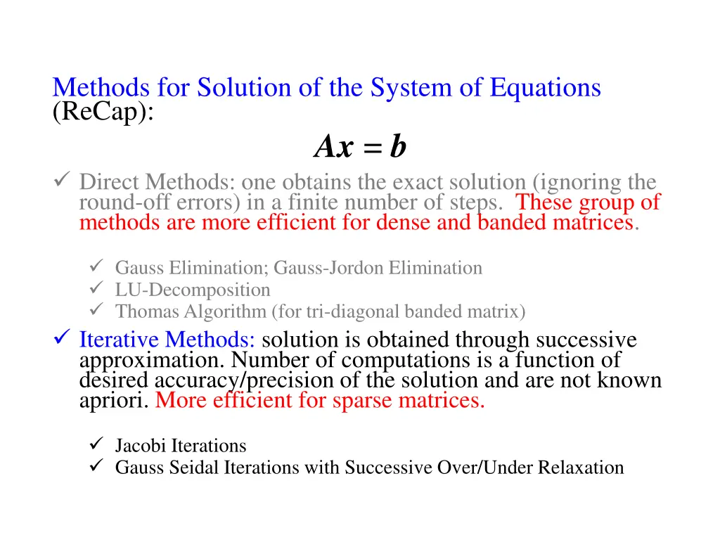
Methods for Solution of the System of Equations (ReCap): Ax = b Direct Methods: one obtains the exact solution (ignoring the round-off errors) in a finite number of steps. These group of methods are more efficient for dense and banded matrices. Gauss Elimination; Gauss-Jordon Elimination LU-Decomposition Thomas Algorithm (for tri-diagonal banded matrix) Iterative Methods: solution is obtained through successive approximation. Number of computations is a function of desired accuracy/precision of the solution and are not known apriori. More efficient for sparse matrices. Jacobi Iterations Gauss Seidal Iterations with Successive Over/Under Relaxation

Sparse Matrix Sparse Matrix 0 0 0 0 0 0 0 0 0 0 0 0 0 0 0 0 0 0 0 0 0 0 0 0 0 0 0 0 0 0 0 0 0 0 0 0 0 0 0 0 0 0 0 0 0 0 0 0 0 0 0 0 0 0 0 0 0 0 0 0 0 0 0 0 Total number of elements = n2 Number of non-zero elements ~ O(n) Direct method algorithms such as Gauss elimination, Gauss Jordon, LU decomposition are inefficient for Banded and Sparse Matrices!

Iterative Methods a11x1 + a12x2 + a13x3 + a1nxn = b1 a21x1 + a22x2 + a23x3 + a2nxn = b2 a31x1 + a32x2 + a33x3 + a3nxn = b3 ai1x1 + ai2x2 + ai3x3 + ainxn = bi an1x1 + an2x2 + an3x3 + annxn = bn Assume (initialize) a solution vector x Compute a new solution vector xnew Iterate until x- xnew We will learn two methods: Jacobi and Gauss Seidel

Jacobi and Gauss Seidel Jacobi: for the iteration index k (k = 0 for the initial guess) b j j k i = n ( ) k a x i ij j , 1 = ) 1 + i ( , 1 = , , 2 x i n a ii Gauss Seidel: for the iteration index k (k = 0 for the initial guess) 1 i = n = ) 1 + ( ( ) k k b a x a 1 x i ij ij j j + ) 1 + 1 j j i ( k = , 1 = , , 2 x i n i a ii

Stopping Criteria Generate the error vector (e) at each iteration as ?+1 ?? ?? ? ?? ?+1= ?? ; ? = 1,2, ? ?+1 Stop when: e Let s review last lecture s example

Iterative methods (Example) Original Problem + = 2 1 x x x A= b= 1 0 0 1 2 1 0 0 0 2 -1 2 -1 0 2 -1 1 1 2 4 + = 2 + 5 . 1 = x x x 1.5 1.5 2 2 3 x 2 x 5 . 1 = x x 3 4 + 2 2 1 3 4 Pivoting: Columns 2 to 1, 3 to 2, 4 to 3 and 1 to 4. After Pivoting A= b= 2 1 0 0 0 2 -1 2 -1 0 2 -1 1 0 0 1 1 This is equivalent to change of variables: x1 (new) = x2 (original) x2 (new) = x3 (original) x3 (new) = x4 (original) x4 (new) = x1 (original) 1.5 1.5 2

Iterative Methods (Example) A= b= 2 1 0 0 0 2 -1 2 -1 0 2 -1 1 0 0 1 1 New Iteration Equations after pivoting (variable identifiers in the subscript are for the new renamed variables): 1.5 1.5 2 ( 3 ) ( 4 ) k k ( ) k + 1 x x 5 . 1 = x ) 1 + ) 1 + ( ( 2 k k 1 = x x 1 2 ( 2 2 Jacobi ( 2 ) ( 3 ) k k ) k + + 2 2 x x 5 . 1 = x ) 1 + ) 1 + ( 3 ( 4 k k = x x 2 ) 1 ) 1 + ( 3 ( 4 ) k k ( k + 1 x x 5 . 1 = x ) 1 + ) 1 + ( ( 2 k k 1 = x x 1 2 ( 2 2 Gauss Seidel ) 1 + ) 1 + ) 1 + ( 2 ( 3 k k k + + 2 2 x x 5 . 1 = x ) 1 + ) 1 + ( 3 ( 4 k k = x x 2 1

Solution: Jacobi Iter 0 1 2 3 4 5 6 7 8 9 10 11 12 13 14 15 16 17 18 19 20 21 22 23 24 25 26 27 28 29 30 31 x1 x2 x3 x4 ||e|| 32 33 34 35 36 37 38 39 40 41 42 43 44 45 46 47 48 49 50 51 52 53 54 55 56 57 58 59 60 61 62 63 64 0.148 0.184 0.151 0.181 0.153 0.179 0.156 0.177 0.157 0.175 0.159 0.174 0.160 0.173 0.161 0.172 0.162 0.171 0.163 0.170 0.164 0.169 0.164 0.169 0.165 0.169 0.165 0.168 0.165 0.168 0.165 0.168 0.166 0.656 0.676 0.658 0.675 0.659 0.673 0.661 0.672 0.662 0.671 0.662 0.671 0.663 0.670 0.664 0.669 0.664 0.669 0.665 0.669 0.665 0.668 0.665 0.668 0.665 0.668 0.666 0.668 0.666 0.667 0.666 0.667 0.666 1.089 1.078 1.088 1.079 1.087 1.080 1.087 1.080 1.086 1.081 1.086 1.081 1.085 1.082 1.085 1.082 1.085 1.082 1.084 1.082 1.084 1.082 1.084 1.083 1.084 1.083 1.084 1.083 1.084 1.083 1.084 1.083 1.084 1.721 1.777 1.726 1.772 1.730 1.768 1.733 1.765 1.736 1.763 1.738 1.761 1.740 1.759 1.742 1.757 1.743 1.756 1.744 1.755 1.745 1.754 1.746 1.754 1.747 1.753 1.747 1.753 1.748 1.752 1.748 1.752 1.748 3.529 3.131 2.940 2.612 2.449 2.186 2.035 1.827 1.697 1.525 1.413 1.275 1.177 1.064 0.982 0.888 0.818 0.742 0.682 0.619 0.569 0.516 0.474 0.431 0.395 0.360 0.330 0.300 0.275 0.250 0.229 0.209 0.191 65 66 67 68 69 70 71 72 73 74 75 76 77 78 79 80 81 82 83 84 85 86 87 88 89 90 91 92 93 94 95 96 97 0.168 0.166 0.167 0.166 0.167 0.166 0.167 0.166 0.167 0.166 0.167 0.166 0.167 0.166 0.167 0.166 0.167 0.166 0.167 0.166 0.167 0.167 0.167 0.167 0.167 0.167 0.167 0.167 0.167 0.167 0.167 0.167 0.167 0.667 0.666 0.667 0.666 0.667 0.666 0.667 0.666 0.667 0.666 0.667 0.666 0.667 0.667 0.667 0.667 0.667 0.667 0.667 0.667 0.667 0.667 0.667 0.667 0.667 0.667 0.667 0.667 0.667 0.667 0.667 0.667 0.667 1.083 1.084 1.083 1.084 1.083 1.084 1.083 1.083 1.083 1.083 1.083 1.083 1.083 1.083 1.083 1.083 1.083 1.083 1.083 1.083 1.083 1.083 1.083 1.083 1.083 1.083 1.083 1.083 1.083 1.083 1.083 1.083 1.083 1.751 1.749 1.751 1.749 1.751 1.749 1.751 1.749 1.751 1.749 1.751 1.749 1.750 1.750 1.750 1.750 1.750 1.750 1.750 1.750 1.750 1.750 1.750 1.750 1.750 1.750 1.750 1.750 1.750 1.750 1.750 1.750 1.750 0.174 0.159 0.145 0.133 0.121 0.111 0.101 0.093 0.084 0.077 0.070 0.064 0.059 0.054 0.049 0.045 0.041 0.037 0.034 0.031 0.028 0.026 0.024 0.022 0.020 0.018 0.017 0.015 0.014 0.013 0.011 0.010 0.010 0.000 0.500 -0.125 0.438 -0.063 0.391 -0.039 0.344 -0.002 0.323 0.030 0.294 0.048 0.271 0.070 0.257 0.086 0.240 0.098 0.228 0.111 0.219 0.120 0.209 0.127 0.203 0.134 0.197 0.139 0.192 0.144 0.188 0.000 0.750 0.500 0.813 0.531 0.781 0.555 0.770 0.578 0.751 0.588 0.735 0.603 0.726 0.614 0.715 0.622 0.707 0.630 0.701 0.636 0.695 0.641 0.690 0.645 0.686 0.649 0.683 0.652 0.680 0.654 0.678 0.000 0.750 1.125 1.000 1.156 1.016 1.141 1.027 1.135 1.039 1.125 1.044 1.117 1.051 1.113 1.057 1.108 1.061 1.103 1.065 1.100 1.068 1.097 1.070 1.095 1.073 1.093 1.074 1.091 1.076 1.090 1.077 0.000 2.000 1.250 2.125 1.375 2.094 1.453 2.031 1.488 1.979 1.537 1.949 1.574 1.912 1.599 1.885 1.627 1.864 1.647 1.844 1.663 1.829 1.679 1.816 1.690 1.804 1.700 1.796 1.708 1.788 1.715 1.782 60.000 41.176 54.545 34.328 44.086 28.462 36.483 24.778 28.717 21.123 23.771 17.637 19.537 15.143 15.827 12.734 13.200 10.664 10.858 9.054 8.940 7.568 7.458 6.344 6.157 5.344 5.110 4.458 4.260 3.736 Number of iteration required to achieve a relative error of < 0.01% = 97

Solution: Gauss Seidel Iter 0 1 2 3 4 5 6 7 8 9 10 11 12 13 14 x1 x2 x3 x4 ||e|| 0.000 0.500 0.000 0.250 0.125 0.188 0.156 0.172 0.164 0.168 0.166 0.167 0.167 0.167 0.167 0.000 0.500 0.750 0.625 0.688 0.656 0.672 0.664 0.668 0.666 0.667 0.667 0.667 0.667 0.667 0.000 1.000 1.125 1.063 1.094 1.078 1.086 1.082 1.084 1.083 1.083 1.083 1.083 1.083 1.083 0.000 2.000 1.625 1.813 1.719 1.766 1.742 1.754 1.748 1.751 1.750 1.750 1.750 1.750 1.750 30.769 13.793 7.273 3.540 1.794 0.891 0.447 0.223 0.112 0.056 0.028 0.014 0.007 Number of iteration required to achieve a relative error of < 0.01% = 14 So, what makes the methods diverge? When do we need pivoting or scaling or equilibration for the iterative methods? Let s analyze for the convergence criteria!

Questions? What are the conditions of convergence for the iterative methods? Rate of convergence? Can we make them converge faster?

Iterative Methods a a a x b 11 12 1 1 1 n a a a x b 21 22 2 2 2 n = a a a x b 31 32 3 3 3 n a a a x b 1 2 m m mn n m How the iteration schemes look in the matrix form ?

Iterative Methods A L 0 a 0 0 a a a 11 12 1 n = + 0 0 a 0 0 a a a 21 22 2 21 n 0 0 a a a a 31 32 3 31 32 n 0 a a a a a a 1 2 1 2 3 n n nn n n n D U 0 0 0 a 0 0 a a a 11 12 13 1 n + 0 0 0 a 0 0 0 a a 22 23 2 n 0 0 0 a 0 0 0 a 33 3 n 0 0 0 0 a 0 0 nn

Iterative Methods A = L + D + U Ax = b translates to (L + D + U)x = b Jacobi: for an iteration counter k ) 1 + ) 1 + ( ( ( ( ) ) k k k k = = + + + + U ( ) ) U ( Dx Dx L L x x b b ) 1 + ) 1 + ( ( 1 1 ( ( ) ) 1 1 k k k k = = + + + + U ( U ( ) ) x x D D L L x x D D b b Gauss Seidel: for an iteration counter k ) 1 + ) 1 + ( ( ( ( ) ) k k k k + + = = + + ( ( ) ) L L D D x x Ux 1 ) b b Ux ) 1 + ) 1 + ( ( 1 ( ( ) ) 1 1 k k k k = = + + + + + + ( ( ) ( ( ) ) x x L L D D Ux Ux L L D D b b

Iterative Methods: Convergence + ( ) 1 ( ) k k = + For all iterative methods: x Sx c 1 1 = + = U ( ) S D L c D b Jacobi: 1 1 = + = + ( ) ( ) S L D U c L D b Gauss Seidel: For true solution vector (x): x = Sx+c True error: e(k) = x- x(k) e(k+1) = x- x(k+1) = (Sx+c) (Sx(k)+c) = Se(k) This constant matrix S governs whether error at each iteration step will increase or decrease: Stationery Iterative Methods Thus, e(k) = Ske(0) lim lim ( ) k k = = 0 0 S e Methods will converge if: k k

Iterative Methods: Convergence For the solution to exist, the matrix should have full rank (= n) The iteration matrix S will have n eigenvalues and n independent eigenvectors that will form the basis for an n-dimensional vector space Initial error vector: e = n j = 1 j n j v = 1 j n = ) 0 ( C jv j 1 j From the definition of eigenvalues: Svj = jvj ?(?) =???(0)=?? ?=1 n = ? ( ) k k j ? ? ? ? = e C v j j 1 j Necessary condition: Spectral Radius, (S) < 1 Sufficient condition: because S ( ) A A 1

Defining Vector and Matrix Norms 16

Vector Norms: A vector norm is a measure (in some sense) of the size or length of a vector Properties of Vector Norm: ? > 0 for ? ?; ? = 0 iff ? = ? ?? = ? ? for a scalar ? ? + ? ? + ? Lp-Norm of a vector x: 1? ?+ ?2 ? + ?? ? ??= ?1 Example Norms: p = 1: sum of the absolute values p = 2: Euclidean norm p : maximum absolute value, ? = max 0 ? ???

Matrix Norms: A matrix norm is a measure of the size of a matrix Properties of Matrix norm: ? > 0 for ? ?; ? = 0 iff ? = ? ?? = ? ? for a scalar ? ? + ? ? + ? ?? ? ? ?? ? ?for consistent matrix and vector norms Lp Norm of a matrix A: ??? ?? ??= max ? ? Spectral Radius: largest absolute eigenvalue of matrix A denoted by (A) If there are m distinct eigenvalues of A: ? ? = max Lower bound of all matrix norms:? ? ? For any norm of matrix A:? ? = lim 1 ? ??? 1? ? ??

Matrix Norms: ? Column-Sum norm: ?1= max 1 ? ? ?=1 ??? 12where, j are the Spectral norm: ?2= eigenvalues of the square symmetric matrix ATA. max 1 ? ??? ? Row-Sum norm: ? = max 1 ? ? ?=1 ??? ? ?=1 ? 2= Frobenius norm: ??= trace ??? ?=1 ??? Trace of a matrix is the sum of elements on the main diagonal

Coming back to Convergence of Iterative Methods 20

Iterative Methods: Convergence For the solution to exist, the matrix should have full rank (= n) The iteration matrix S will have n eigenvalues and n independent eigenvectors that will form the basis for an n-dimensional vector space Initial error vector: e = n j = 1 j n j v = 1 j n = ) 0 ( C jv j 1 j From the definition of eigenvalues: Svj = jvj ?(?) =???(0)=?? ?=1 n = ? ( ) k k j ? ? ? ? = e C v j j 1 j Necessary condition: Spectral Radius, (S) < 1 Sufficient condition: because S ( ) A A 1

Jacobi Convergence -aij aii for i j S = - D-1(L+U) sij= 0 for i = j If we use row-sum norm: max 1 i n Recall, Sufficient Condition for Convergence: S n n aij aii max 1 i n S = sij= j=1 j=1 1 n aii> , i =1,2, n aij j=1,j i

Iterative Methods: Convergence Using the definition of S and using row-sum norm for matrix S, we obtain the following as the sufficient condition for convergence for both Jacobi and Gauss Seidel: n = = , , 2 , 1 a a i i n ii ij , 1 j j If the original matrix is diagonally dominant, it will always converge!

Rate of Convergence For large k: ??+1 ?? ? ? or ?? ?0 ? ?? Why?

Rate of Convergence Number of iterations (k) required to decrease the initial error by a factor of 10-m is then given by: ?? ?0 ? ??= 10 ? or ? ? =? ? = log10? ? log10? ? ? R is the asymptotic rate of convergence of the iterative methods.

Improving Convergence Recall Gauss Seidel: 1 i = n = ) 1 + ( ( ) k k b a x a 1 x i ij ij j j + ) 1 + 1 j j i ( k = , 1 = , , 2 x i n i a ii Re-Write As: i-1 n (k+1)- bi- (k) aijxj aijxj j=1 j=i (k+1)= xi (k)+ , i =1, 2, n xi aii (k+1)= xi (k)+di (k), i=1, 2, n xi

Improving Convergence r S ( )= lmax Denoting: e(k+1)@ lmaxe(k) or e(k+1)-e(k)@ lmax(e(k)-e(k-1)) For any iterative method: x(k+1) = x(k) + d(k) d(k)@lmaxd(k-1)

Successive Over/Under Relaxation (k+1)= xi (k)+wdi (k), i=1, 2, n, w >0 xi 0 < < 1 : Under relaxation = 1 : Gauss Seidel 1 < < 2 : Over Relaxation i-1 n (k+1)- bi- (k) aijxj aijxj j=1 j=i+1 (k+1)=(1-w)xi (k)+w , i =1, 2, n xi aii

Pivoting, Scaling and Equilibration, Perturbation Analysis

Recall Gauss Elimination: Step 1: k = 1 ??1= i= 2, 3, .n and j= 2, 3, n ??1 ?11; ???= ???-??1?1?; ??= ?? ??1 ?1 Step 2: k = 2 ??2= i= 3, 4, .n and j= 3, 4, n ??2 ?22; ???= ???-??2?2?; ??= ?? ??2 ?2 Step k: k = k ???= i = k+1, k+2, .n and j = k+1, k+2, .n ??? ???; ???= ???-??????; ??= ?? ??? ?? for At each k, the all the elements in rows > k are multiplied by lik. Roundoff errors will be magnified and eventually may grow out of bound if lik > 1 (i.e., algorithm become unstable) Condition for stability: lik 1 (for all k) This will happen only if akk is the largest element in the kth column for rows k If not, make it! (This operation is called pivoting)

Partial Pivoting: Matrix at the start of the kth Step: Row Exchange apk Before operations of the kth step, Search for max interchange kth row with the pth row Interchange the right hand side vector bk with bp, if not working with the augmented matrix.) ? ? ????. Let s say, it occurs at i = p

Full Pivoting: Matrix at the start of the kth Step: Column Exchange Row Exchange apq Before operations of the kth step, Search for max ? ? ? ? ? ? interchange kth row with pth row, kth column with the qth column Interchange the right hand side vector bk with bp, if not working with the augmented matrix.) Column interchange renaming of variables k ???. Let s say, it occurs at i = p; j = q q

Perturbation Analysis Consider the system of equation Ax = b Question: If small perturbation is given in the matrix A and/or the vector b, what is the effect on the solution vector x ? Alternatively, how sensitive is the solution to small perturbations in the coefficient matrix and the forcing function. R1 = 10.0 1.2 ; R2 = 15.0 1.8 ; R3 = 25.0 2.7 VA - VC = 100.0 11.0 V; VA - VB= 60.0 9.0 V Example: C Let s denote the resulting perturbation in the solution vector x as x R3 B i3 R1 A A i1 b b i2 ?1 ?2 ?3 0 0 0 0 0 1 0 10 1 15 15 1 25 0 0 + 1.8 1.8 2.7 0 = + 11 9 100 60 R2 1.2 A

Perturbation in matrix A: System of equation: (A + A)(x + x)= b A x + A(x + x)=0 since, Ax = b x =- A-1 A(x + x) Take the norms of vectors and matrices: ?? = ? ??? ? + ?? ? ? ? ? ?? ?? ? + ?? ?? ? + ? ? ?? Product of perturbation quantities ?? ? ?? ? ? ? ?

Perturbation in forcing vector b: System of equation: A(x + x)=(b + b) A x = b since, Ax = b x =- A-1 b Take the norms of vectors and matrices: ?? ? ?? = ? ??? ? ? ?? = ? ? ? ?? ? ? ? ? ? ?? ? ?? ? ? ? ?

Condition Number: Condition number of a matrix A is defined as: ? ? = ? ? ? ? ?is the proportionality constant relating relative error or perturbation in A and b with the relative error or perturbation in x Value of ? ? depends on the norm used for calculation. Use the same norm for both A and A-1. If ? ? 1 or of the order of 1, the matrix is well- conditioned. If ? ? 1 , the matrix is ill-conditioned.

Scaling and Equilibration: It helps to reduce the truncation errors during computation. Helps to obtain a more accurate solution for moderately ill- conditioned matrix. Example: Consider the following set of equation Scale variable x1 = 103 x1 and multiply the second equation by 100. Resulting equation is:

Scaling Vector x is replaced by x such that, x = Sx . S is a diagonal matrix containing the scale factors! For the example problem: Ax = b becomes: Ax = ASx = A x = b where, A = AS For the example problem: Scaling operation is equivalent to post-multiplication of the matrix A by a diagonal matrix S containing the scale factors on the diagonal

Equilibration Equilibration is multiplication of one equation by a constant such that the values the coefficients become same order of magnitude as the other equations. The operation is equivalent to pre-multiplication by a diagonal matrix E on both sides of the equation. Ax = b becomes: EAx = Eb For the example problem: 1 0 0 0 102 0 0 0 1 0.0015 0.966 0.003 1.45 0.002 0.96 0.0015 0.966 Equilibration operation is equivalent to pre-multiplication of the matrix A and vector b by a diagonal matrix E containing the equilibration factors on the diagonal ?1 ?2 ?3 ?1 ?2 ?3 1 0 0 0 0 0 1 11 0.12 19 0.003 0.00002 1.45 0.0096 0.3 102 0 = 0.0021 0.201 0.3 0.21 0.201 11 12 19 =

Pivoting, Scaling and Equilibration Before starting the solution algorithm, take a look at the entries in A and decide on the scaling and equilibration factors. Construct matrices E and S. Transform the set of equation Ax = b to EASx = Eb Solve the system of equation A x = b for x , where A = EAS and b = Eb Compute: x = Sx Gauss Elimination: perform partial pivoting at each step k For all other methods: perform full pivoting before the start of the algorithm to make the matrix diagonally dominant, as far as practicable! These steps will guarantee the best possible solution for all well- conditioned and mildly ill-conditioned matrices! However, none of these steps can transform an ill-conditioned matrix to a well-conditioned one.

Iterative Improvement by Direct Methods For moderately ill-conditioned matrices an approximate solution x to the set of equation Ax = b can be improved through iterations using direct methods. Compute: r = b - Ax Recognize: r = b - Ax + Ax - b Therefore: A(x - x ) = A x = r Compute: x = x + x The iteration sequence can be repeated until x