Space-Time Tradeoffs & Hash Tables Review
Delve into space-time tradeoffs, Hash tables, and string search algorithms in this insightful discussion. Topics covered include Horner's Rule, problem reduction strategies, finding least common multiples using GCD, paths and adjacency matrices in graphs, and examples showcasing the tradeoffs between space and time in algorithm design.

Download Presentation

Please find below an Image/Link to download the presentation.
The content on the website is provided AS IS for your information and personal use only. It may not be sold, licensed, or shared on other websites without obtaining consent from the author.If you encounter any issues during the download, it is possible that the publisher has removed the file from their server.
You are allowed to download the files provided on this website for personal or commercial use, subject to the condition that they are used lawfully. All files are the property of their respective owners.
The content on the website is provided AS IS for your information and personal use only. It may not be sold, licensed, or shared on other websites without obtaining consent from the author.
E N D
Presentation Transcript
MA/CSSE 473 Day 24 Student questions Space-time tradeoffs Hash tables review String search algorithms intro
We did not get to them in other sections THINGS WE DID LAST TIME IN SECTION 1
Horner's Rule It involves a representation change. Instead of anxn + an-1xn-1+ . + a1x + a0, which requires a lot of multiplications, we write ( (anx + an-1)x + +a1 )x + a0 code on next slide
Horner's Rule Code This is clearly (n).
Problem Reduction Express an instance of a problem in terms of an instance of another problem that we already know how to solve. There needs to be a one-to-one mapping between problems in the original domain and problems in the new domain. Example: In quickhull, we reduced the problem of determining whether a point is to the left of a line to the problem of computing a simple 3x3 determinant. Example: Moldy chocolate problem in HW 9. The big question: What problem to reduce it to? (You'll answer that one in the homework)
Least Common Multiple Let m and n be integers. Find their LCM. Factoring is hard. But we can reduce the LCM problem to the GCD problem, and then use Euclid's algorithm. Note that lcm(m,n) gcd(m,n) = m n This makes it easy to find lcm(m,n)
Paths and Adjacency Matrices We can count paths from A to B in a graph by looking at powers of the graph's adjacency matrix. For this example, I used the applet from http://oneweb.utc.edu/~Christopher-Mawata/petersen2/lesson7.htm, which is no longer accessible
Sometimes using a little more space saves a lot of time SPACE-TIME TRADEOFFS
Space vs time tradeoffs Often we can find a faster algorithm if we are willing to use additional space. Give some examples Examples:
Space vs time tradeoffs Often we can find a faster algorithm if we are willing to use additional space. Give some examples (quiz question) Examples: Binary heap vs simple sorted array. Uses one extra array position Merge sort Sorting by counting Radix sort and Bucket Sort Anagram finder Binary Search Tree (extra space for the pointers) AVL Tree (extra space for the balance code)
A Quick Review HASH TABLE IMPLEMENTATION
Hash Table Review Section 7.4 of Levitin Excellent detailed reference: Weiss Chapter 20. Covered in 230 Both versions of the course A link to one version: http://www.rose- hulman.edu/class/csse/csse230/201230/Slides/17-Graphs- HashTables.pdf Three questions on today's handout guide you through a quick review; the above link may be helpful. Do it with two other students. 20 minutes. Then we will prove a property of quadratic probing that is described in 230 but seldom proved there. If you don't understand the effects of clustering, you might find the animation that is linked from this page to be especially helpful. : http://www.cs.auckland.ac.nz/software/AlgAnim/hash_tables.html
Collision Resolution: Quadratic probing With linear probing, if there is a collision at H, we try H, H+1, H+2, H+3, ... (all modulo the table size) until we find an empty spot. Causes (primary) clustering With quadratic probing, we try H, H+12. H+22, H+32, ... Eliminates primary clustering, but can cause secondary clustering. Is it possible that it misses some available array positions? I.e it repeats the same positions over and over, while never probing some other positions?
Hints for quadratic probing Choose a prime number for the array size, then If the array is not more than half full, finding a place to do an insertion is guaranteed , and no cell is probed twice before finding it Suppose the array size is P, a prime number greater than 3 Show by contradiction that if i and j are P/2 , and if i j, then H + i2 (mod P) H + j2 (mod P). Use an algebraic trick to calculate next index Replaces mod and general multiplication with subtraction and a bit shift Difference between successive probes: H + (i+1)2 = H + i2 + (2i+1) [can use a bit-shift for the multiplication]. nextProbe = nextProbe + (2i+1); if (nextProbe >= P) nextProbe -= P;
Quadratic probing analysis No one has been able to analyze it Experimental data shows that it works well Provided that the array size is prime, and is the table is less than half full
Hashing Highlights (consider this later) We cover this pretty thoroughly in CSSE 230, and Levitin does a good job of reviewing it concisely, so I'll have you read it on your own (section 7.3). On the next slides you'll find a list of things you should know (some of them expressed here as questions) Details in Levitin section 7.3 and Weiss chapter 20. Outline of what you need to know is on the next slides. Will not cover them in great detail in class, since they are typically covered well in 230.
Hashing You should know, part 1 Hash table logically contains key-value pairs. Represented as an array of size m. H[0..m-1] Typically m is larger than the number of pairs currently in the table. Hash function h(K) takes key K to a number in range 0..m Hash function goals: Distribute keys as evenly as possible in the table. Easy to compute. Does not require m to be a lot larger than the number of keys in the table.
Hashing You should know, part 2 Load factor: ratio of used table slots to total table slots. Smaller better time efficiency (fewer collisions) Larger better space efficiency Two main approaches to collision resolution Open addressing Se Open addressing basic idea When there is a collision during insertion, systematically check later slots (with wraparound) until we find an empty spot. When searching, we systematically move through the array in the same way we did upon insertion until we find the key we are looking for or an empty slot.
Hashing You should know, part 3 Open addressing linear probing When there is a collision, check the next cell, then the next one, , (with wraparound) Let be the load factor, and let S and U be the expected number of probes for successful and unsuccessful searches. Expected values for S and U are
Hashing You should know, part 4 Open addressing double hashing When there is a collision, use another hash function s(K) to decide how much to increment by when searching for an empty location in the table So we look in H(k), H(k) + s(k), H(k) + 2s(k), , with everything being done mod m. If we we want to utilize all possible array positions, gcd(m, s(k)) must be 1. If m is prime, this will happen.
Hashing You should know, part 5 Separate chaining Each of the m positions in the array contains a link ot a structure (perhaps a linked list) that can hold multiple values. Does not have the clustering problem that can come from open addressing. For more details, including quadratic probing, see Weiss Chapter 20 or my CSSE 230 slides (linked from the schedule page)
Search for a string within another string STRING SEARCH
Brute Force String Search Example The problem: Search for the first occurrence of a pattern of length m in a text of length n. Usually, m is much smaller than n. What makes brute force so slow? When we find a mismatch, we can shift the pattern by only one character position in the text. Text: Pattern:abracadabra abracadabra abracadabra abracadabra abracadabra abracadabra abracadabtabradabracadabcadaxbrabbracadabraxxxxxxabracadabracadabra
Faster String Searching Was a HW problem Brute force: worst case m(n-m+1) A little better: but still (mn) on average Short-circuit the inner loop
Horspool's Algorithm Intro A simplified version of the Boyer-Moore algorithm A good bridge to understanding Boyer-Moore Published in 1980 What makes brute force so slow? When we find a mismatch, we can only shift the pattern to the right by one character position in the text. Text: abracadabtabradabracadabcadaxbrabbracadabraxxxxxxabracadabracadabra Pattern:abracadabra abracadabra abracadabra abracadabra Can we shift farther? Like Boyer-Moore, Horspool does the comparisons in a counter-intuitive order (moves right-to-left through the pattern)
Horspool's Main Question If there is a character mismatch, how far can we shift the pattern, with no possibility of missing a match within the text? What if the last character in the pattern is compared with a character in the text that does not occur in the pattern at all? Text: ... ABCDEFG ... Pattern: CSSE473
How Far to Shift? Look at first (rightmost) character in the part of the text that is compared to the pattern: The character is not in the pattern .....C.......... {C not in pattern) BAOBAB The character is in the pattern (but not the rightmost) .....O..........(O occurs once in pattern) BAOBAB .....A..........(A occurs twice in pattern) BAOBAB The rightmost characters do match .....B...................... BAOBAB


")