Sparse Matrix Algorithms: Permutations and Chordal Completion
Most coefficients in matrices are zero, leading to sparsity. Sparse Gaussian elimination and chordal completion aim to minimize edges while solving matrices efficiently. The 2D model problem illustrates behaviors of sparse matrix algorithms. Permutations impact fill levels, with natural and nested dissection permutations showing distinct fill orders. Nested dissection ordering segregates vertices based on separators for efficient graph processing.
Download Presentation

Please find below an Image/Link to download the presentation.
The content on the website is provided AS IS for your information and personal use only. It may not be sold, licensed, or shared on other websites without obtaining consent from the author.If you encounter any issues during the download, it is possible that the publisher has removed the file from their server.
You are allowed to download the files provided on this website for personal or commercial use, subject to the condition that they are used lawfully. All files are the property of their respective owners.
The content on the website is provided AS IS for your information and personal use only. It may not be sold, licensed, or shared on other websites without obtaining consent from the author.
E N D
Presentation Transcript
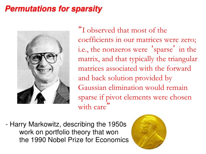
Permutations for sparsity I observed that most of the coefficients in our matrices were zero; i.e., the nonzeros were sparse in the matrix, and that typically the triangular matrices associated with the forward and back solution provided by Gaussian elimination would remain sparse if pivot elements were chosen with care - Harry Markowitz, describing the 1950s work on portfolio theory that won the 1990 Nobel Prize for Economics
Sparse Gaussian elimination and chordal completion [Parter, Rose] Repeat: Choose a vertex v and mark it; Add edges between unmarked neighbors of v; Until: Every vertex is marked Goal: End up with as few edges as possible. Equivalently: Add as few edges as possible to make the graph chordal. (Note for later: Fewest edges is not the only interesting objective.)
The (2-dimensional) model problem n1/2 Graph is a regular square grid with n = k2 vertices. Corresponds to matrix for regular 2D finite difference mesh. Gives good intuition for behavior of sparse matrix algorithms on many 2-dimensional physical problems. There s also a 3-dimensional model problem.
Permutations of the 2-D model problem Theorem 1: With the natural permutation, the n-vertex model problem has exactly O(n3/2) fill. Theorem 2: With a nested dissection permutation, the n-vertex model problem has exactly O(n log n) fill. Theorem 3: With any permutation, the n-vertex model problem has at least O(n log n) fill. See course notes for proofs.
Nested dissection ordering A separator in a graph G is a set S of vertices whose removal leaves at least two connected components. A nested dissection ordering for an n-vertex graph G numbers its vertices from 1 to n as follows: Find a separator S, whose removal leaves connected components T1, T2, , Tk Number the vertices of S from n-|S|+1 to n. Recursively, number the vertices of each component: T1 from 1 to |T1|, T2 from |T1|+1 to |T1|+|T2|, etc. If a component is small enough, number it arbitrarily. It all boils down to finding good separators!
Separators in theory If G is a planar graph with n vertices, there exists a set of at most sqrt(6n) vertices whose removal leaves no connected component with more than 2n/3 vertices. ( Planar graphs have sqrt(n)-separators. ) Well-shaped finite element meshes in 3 dimensions have n2/3 - separators. Also some other classes of graphs trees, graphs of bounded genus, chordal graphs, bounded-excluded- minor graphs, Mostly these theorems come with efficient algorithms, but they aren t used much.
Separators in practice Graph partitioning heuristics have been an active research area for many years, often motivated by partitioning for parallel computation. See CS 240A. Some techniques: Spectral partitioning (uses eigenvectors of Laplacian matrix of graph) Geometric partitioning (for meshes with specified vertex coordinates) Iterative-swapping (Kernighan-Lin, Fiduccia-Matheysses) Breadth-first search (fast but dated) Many popular modern codes (e.g. Metis, Chaco) use multilevel iterative swapping Matlab graph partitioning toolbox: see course web page
Permutations of general 2D and 3D problems Theorem 4: With a nested dissection permutation, any planar graph with n vertices has at most O(n log n) fill. Theorem 5: With a nested dissection permutation, any 3D finite element mesh (with a technical condition on element shapes) has at most O(n 4/3 ) fill. See course notes for references to proofs.
Heuristic fill-reducing matrix permutations Nested dissection: Find a separator, number it last, proceed recursively Theory: approx optimal separators => approx optimal fill and flop count Practice: often wins for very large problems Minimum degree: Eliminate row/col with fewest nzs, add fill, repeat Hard to implement efficiently current champion is Approximate Minimum Degree [Amestoy, Davis, Duff] Theory: can be suboptimal even on 2D model problem Practice: often wins for medium-sized problems Banded orderings (Reverse Cuthill-McKee, Sloan, . . .): Try to keep all nonzeros close to the diagonal Theory, practice: often wins for long, thin problems The best modern general-purpose orderings are ND/MD hybrids.
Fill-reducing permutations in Matlab Symmetric approximate minimum degree: p = amd(A); symmetric permutation: chol(A(p,p)) often sparser than chol(A) Symmetric nested dissection: not built into Matlab several versions in meshpart toolbox (course web page references) Nonsymmetric approximate minimum degree: p = colamd(A); column permutation: lu(A(:,p)) often sparser than lu(A) also for QR factorization Reverse Cuthill-McKee p = symrcm(A); A(p,p) often has smaller bandwidth than A similar to Sparspak RCM
Complexity of direct methods Time and space to solve any problem on any well- shaped finite element mesh n1/2 n1/3 2D 3D O(n log n) O(n 4/3 ) Space (fill): O(n 3/2 ) O(n 2 ) Time (flops):
Compressed Sparse Matrix Storage value (x in Davis) : 31 41 59 26 53 31 0 53 row (i in Davis) : 1 3 2 3 1 0 59 0 41 26 0 colstart (p in Davis) : 1 3 5 6 Sparse storage: Compressed storage by columns (CSC). Three 1-dimensional arrays. (2*nzs + ncols + 1) memory. Similarly, CSR. Full storage: 2-dimensional array. (nrows*ncols) memory.
Matrix Matrix Multiplication: C = A * B C(:, :) = 0; for i = 1:n for j = 1:n for k = 1:n C(i, j) = C(i, j) + A(i, k) * B(k, j); The n3 scalar updates can be done in any order. Six possible algorithms: ijk, ikj, jik, jki, kij, kji (lots more if you think about blocking for cache). Goal is O(nonzero flops) time for sparse A, B, C. Even time = O(n2) is too slow!
Organizations of Matrix Multiplication Barriers to O(flops) work Outer product: for k = 1:n C = C + A(:, k) * B(k, :) - Inserting updates into C is too slow Inner product: for i = 1:n for j = 1:n C(i, j) = A(i, :) * B(:, j) - n2 loop iterations cost too much if C is sparse Column by column: for j = 1:n for k where B(k, j) 0 C(:, j) = C(:, j) + A(:, k) * B(k, j) - Loop k only over nonzeros in column j of B - Use sparse accumulator (SPA) for column updates
CSC Sparse Matrix Multiplication with SPA for j = 1:n C(:, j) = A * B(:, j) x = B C A All matrix columns and vectors are stored compressed except the SPA. scatter/ accumulate gather SPA
Sparse Accumulator (SPA) Abstract data type for a single sparse matrix column Operations: initialize spa spa = spa + (scalar) * (CSC vector) O(nnz(vector)) time (CSC vector) = spa O(nnz(spa)) time spa = 0 O(nnz(spa)) time possibly other ops O(n) time & O(n) space
Sparse Accumulator (SPA) Abstract data type for a single sparse matrix column Operations: initialize spa spa = spa + (scalar) * (CSC vector) O(nnz(vector)) time (CSC vector) = spa O(nnz(spa)) time spa = 0 O(nnz(spa)) time possibly other ops O(n) time & O(n) space Standard implementation (many variants): dense n-element floating-point array value dense n-element boolean array is-nonzero linked structure to sequence through nonzeros
CSC Sparse Matrix Multiplication with SPA for j = 1:n C(:, j) = A * B(:, j) x = B C A All matrix columns and vectors are stored compressed except the SPA. scatter/ accumulate gather SPA
Triangular solve: x = L \ b Column oriented: Row oriented: x(1:n) = b(1:n); for j = 1 : n x(j) = x(j) / L(j, j); x(j+1:n) = x(j+1:n) L(j+1:n, j) * x(j); end; for i = 1 : n x(i) = b(i); for j = 1 : (i-1) x(i) = x(i) L(i, j) * x(j); end; x(i) = x(i) / L(i, i); end; Either way works in O(nnz(L)) time [details for rows: exercise] If b and x are dense, flops = nnz(L) so no problem If b and x are sparse, how do it in O(flops) time?
Directed Graph 2 1 4 5 7 6 3 A G(A) A is square, unsymmetric, nonzero diagonal Edges from rows to columns Symmetric permutations PAPT
Directed Acyclic Graph 2 1 4 5 7 6 3 A G(A) If A is triangular, G(A) has no cycles Lower triangular => edges from higher to lower #s Upper triangular => edges from lower to higher #s
Directed Acyclic Graph 2 1 4 5 7 6 3 A G(A) If A is triangular, G(A) has no cycles Lower triangular => edges from higher to lower #s Upper triangular => edges from lower to higher #s
Depth-first search and postorder dfs (starting vertices) marked(1 : n) = false; p = 1; for each starting vertex v do visit(v); visit (v) if marked(v) then return; marked(v) = true; for each edge (v, w) do visit(w); postorder(v) = p; p = p + 1; When G is acyclic, postorder(v) > postorder(w) for every edge (v, w)
Depth-first search and postorder dfs (starting vertices) marked(1 : n) = false; p = 1; for each starting vertex v do if not marked(v) then visit(v); visit (v) marked(v) = true; for each edge (v, w) do if not marked(w) then visit(w); postorder(v) = p; p = p + 1; When G is acyclic, postorder(v) > postorder(w) for every edge (v, w)
Sparse Triangular Solve 1 1 2 3 4 5 3 5 = 2 4 G(LT) L x b 1. Symbolic: Predict structure of x by depth-first search from nonzeros of b 2. Numeric: Compute values of x in topological order Time = O(flops)
Sparse-sparse triangular solve: x = L \ b Column oriented: dfs in G(LT) to predict nonzeros of x; x(1:n) = b(1:n); for j = nonzero indices of x in topological order x(j) = x(j) / L(j, j); x(j+1:n) = x(j+1:n) L(j+1:n, j) * x(j); end; Depth-first search calls visit once per flop Runs in O(flops) time even if it s less than nnz(L) or n Except for one-time O(n) SPA setup
