Spatial Autocorrelation Processing Using SeisImager

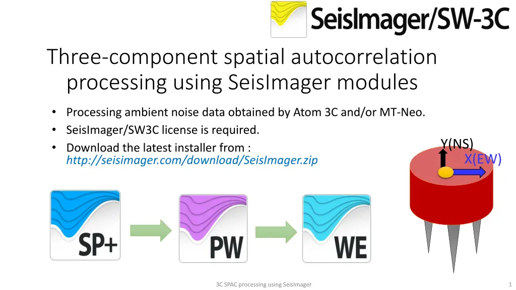
Three-component spatial autocorrelation processing using SeisImager modules Processing ambient noise data obtained by Atom 3C and/or MT-Neo. SeisImager/SW3C license is required. Download the latest installer from : http://seisimager.com/download/SeisImager.zip Y(NS) X(EW) 1 3C SPAC processing using SeisImager

Outline of three-component (3C) measurement and processing Rayleigh and Love wave dispersion curves S-wave velocity model 3C ambient noise data 3C measurement 3C spatial autocorrelation X(EW) Radial Z(UD) Love Y(NS) Y(NS) Transverse Z(UD) X(EW) Rayleigh Vertical Vertical component SPAC provides a Rayleigh dispersion curve. Horizontal components (radial and transverse) provide a Love dispersion curve using Rayleigh dispersion curve. Vertical component provides vertical component SPAC. Horizontal components (X and Y) provide radial and transverse component SPACs. 3C measurement provides 3C ambient noise data. Joint inversion of Rayleigh and Love dispersion curves provide an S-wave velocity model. 2 3C SPAC processing using SeisImager

3C ambient noise measurements for SPAC L-shaped array (L3) Triangular array (T4) Arrange the orientation of all sensors to be the same direction 3 3C SPAC processing using SeisImager

Spatial autocorrelation for 3C ambient noise Direction of horizontal components must be consistent throughout all sensors and kept track. Radial and transverse components are defined for each receiver pair. Transverse component Rotate horizontal components (X and Y) to radial and transpose components Y(NS) component Radial component Transverse component Y(NS) component X(EW) component Radial component X(EW) component A function calculating transpose and radial components of SPAC from 3C ambient noise data was implemented in SPACPlus and dPickwin. 4 3C SPAC processing using SeisImager

SW3C option in SeisImager SW3C option should be checked in SeisImagerRegistarioan to use 3C processing functions or joint inversion of Rayleigh and Love waves. 5 3C SPAC processing using SeisImager

Select a CTB including 3C ambient noise data Example of three component data 6 3C SPAC processing using SeisImager

Data example (3C measurements using 14 sensors) Easting [m] 0 217.34 386.02 -257.41 -362.36 -77.33 120.86 129.83 -96.66 38.67 -83.89 256.12 -91.77 25.57 Northing [m] 0 302.07 14.16 -166.41 182.01 408.01 -76.71 31.65 -105.19 132.35 112.35 -315.96 -381.87 -134.09 7 3C SPAC processing using SeisImager

3C SPAC processing flow using SPACPlus, Pickwin and WaveEq WaveEq Pickwin SPACPlus SPAC (vertical) SEG2 file (.coh) Rayleigh phase velocity image Rayleigh dispersion curve 3C SPAC 3C CTB SPAC (radial) SEG2 file (.coh) Love phase velocity image Love dispersion curve SPAC (transverse) SEG2 file (.coh) 8 3C SPAC processing using SeisImager

CTB including 3C ambient noise data by 14 sensors 9 3C SPAC processing using SeisImager

Calculate SPAC for each component Select array geometry. Click Open array file if manual array file will be used. Click to calculate SPAC Select a component to be calculated (selecting vertical component) Select Manual array if manual array will be used. Click OK to calculate SPAC. 10 3C SPAC processing using SeisImager

Individual SPAC for each receiver spacing 11 3C SPAC processing using SeisImager

Calculate dispersion curve for each component Click to calculate dispersion curve Vertical component Dispersion curve from vertical component corresponds to Rayleigh wave dispersion curve. 12 3C SPAC processing using SeisImager

Save coherencies of each component to a SEG2 file Select File , Save SPAC data as SEG2 file to coherencies to a SEG2 file. Use extension .coh to save coherencies. 13 3C SPAC processing using SeisImager

Repeat SPAC calculation for all components Radial component Note that dispersion curves from transverse and radial components do not correspond to Love wave dispersion curve. Transpose component 14 3C SPAC processing using SeisImager

Switch Pickwin to the complete menu Use the Complete menu to process 3C SPAC data. Complete menu Select Option , Menu type , Simple to the menu type from Simple to Complete . Simple menu 15 3C SPAC processing using SeisImager

Import three SPAC files to Pickwin Select File , Option , Append files to import multi files at once. Select three coherency files (vertical, radial and transverse) and click Open . 16 3C SPAC processing using SeisImager

Import three SPAC files to Pickwin Click Yes to continue. Three component (vertical, radial and transverse) SPACs appear. 17 3C SPAC processing using SeisImager

Calculate Rayleigh and Love phase velocity images Click or press Ctrl+D to calculate phase velocity images. Set up transformation parameters as usual. Click Yes to apply 3C SPAC analysis. 18 3C SPAC processing using SeisImager

Calculate Rayleigh and Love phase velocity images Ryleigh wave phase velocity image appears at first. Click to switch Rayleigh/Love phase velocity images. Rayleigh wave Love wave Note that the color scale of Love wave phase velocity image is opposite to Rayleigh wave. 19 3C SPAC processing using SeisImager

Show Rayleigh and Love dispersion curves by WaveEq Click or select Surface wave analysis , Show phase velocity curve (1D) to show dispersion curves by WaveEq. WaveEq launched and Rayleigh wave dispersion curve appears at first. Click to show Love wave dispersion curve. Rayleigh Love 3C SPAC processing using SeisImager 20

Edit dispersion curve and prepare an initial model Comparison of observed and theoretical dispersion curves (fundamental mode). Edit dispersion curves and prepare an initial model as usual. Observed Theoretical Rayleigh Love 21 3C SPAC processing using SeisImager

Comparison of observed and theoretical dispersion curves (Higher modes) Love Rayleigh Amplitude Velocity Amplitude Velocity Observed Averaged (effective) Fundamental 1st 2nd 3rd 4th 5th 22 3C SPAC processing using SeisImager

Joint inversion of Rayleigh and Love waves Joint inversion of Rayleigh and Love waves using non-linear least squares method or Genetic Algorithm (GA) were implemented in WaveEq. Inversions are available in Inversion (LSM) , GA (Vs only) and GA (Vs and thickness) in MASW/MAM (1D) of WaveEq. 23 3C SPAC processing using SeisImager

Joint inversion of Rayleigh and Love waves Numerical example using two layer model Theoretical velocity model for the true velocity model True velocity model Both Rayleigh and Love wave effective modes are different from fundamental modes. 24 3C SPAC

Joint inversion of Rayleigh and Love waves (only fundamental mode) Initial model Inverted result Inversion using non-linear least squares method. Inversion using non-linear least squares method decreased the error between observed and theoretical dispersion curves. 25 3C SPAC

Joint inversion of Rayleigh and Love waves (including higher modes) Initial model Inverted result Inversion using Genetic Algorithm (GA). Inversion using GA decreased the error between observed and theoretical (effective mode) dispersion curves. 26 3C SPAC

Joint inversion of Rayleigh and Love waves (including higher modes) Field data example Initial model Inverted result Inversion using Genetic Algorithm (GA). 27 3C SPAC

Option : Use dispersion curve from transverse component as Love wave Theoretically, phase velocities of transverse component is close to that of Love waves. You may consider dispersion curve of transverse component as that of Love waves. In active methods, dispersion curves obtained from SH measurements can be considered as the dispersion curves of Love waves. S-wave velocity model Rayleigh and Love wave dispersion curves 3C spatial autocorrelation Transverse (or SH measurement) Love Love wave .rst file Vertical (or P-Sv measurement) Rayleigh Rayleigh wave .rst file 28 3C SPAC processing using SeisImager

Option : Select Rayleigh or Love dispersion curve You have a chance to select Rayleigh or Love dispersion curve when launching WaveEq from Pickwin. Rayleigh wave is shown as red Love wave is shown as blue 29 3C SPAC processing using SeisImager

Option : Switch Rayleigh or Love dispersion curve It is possible to switch (or select) Rayleigh or Love dispersion curve. Use MASW/MAM (1D) , Advanced option , Surface wave mode . Love wave is shown as blue Rayleigh wave is shown as red 30 3C SPAC processing using SeisImager

Option : Combine Rayleigh and Love dispersion curves 1) Save Rayleigh and Love wave dispersion curves to individual files. 5) Rayleigh and Love dispersion curves are shown together. 3) Open another (Love/ Rayleigh) file and append it. 2) Open one (Rayleigh/Love) file. 4) Select Yes . 31 3C SPAC processing using SeisImager