Spatial Correlation in Mixed Models Workshop
Explore the principles of randomized block trials with spatial correlation and Tobler's first law of geography. Learn from an example field experiment, delve into randomized complete block models, and understand the analysis using SAS and R libraries. Discover how spatial correlation impacts model outcomes.
Download Presentation

Please find below an Image/Link to download the presentation.
The content on the website is provided AS IS for your information and personal use only. It may not be sold, licensed, or shared on other websites without obtaining consent from the author. If you encounter any issues during the download, it is possible that the publisher has removed the file from their server.
You are allowed to download the files provided on this website for personal or commercial use, subject to the condition that they are used lawfully. All files are the property of their respective owners.
The content on the website is provided AS IS for your information and personal use only. It may not be sold, licensed, or shared on other websites without obtaining consent from the author.
E N D
Presentation Transcript
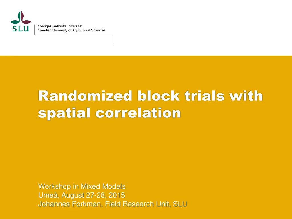
Randomized block trials with spatial correlation Workshop in Mixed Models Ume , August 27-28, 2015 Johannes Forkman, Field Research Unit, SLU
Toblers first law of geography Everything is related to everything else, but near things are more related than distant things Tobler (1970)
Example Field experiment 28 plots in a single row Seven fertilization treatments (A-G) Four blocks 1 2 3 4 5 6 7 8 9 10 11 12 13 14 15 16 17 18 19 20 21 22 23 24 25 26 27 28 C A G D E F B G E B C A F D B A G E D F C E A C F G B D Example provided by Anders Ericsson, Swedish Rural Economy and Agricultural Societies, HS Konsult
Randomized complete block model Yield = Treatment + Block + Error Fixed effects of Treatment Random effects of Block and Error Errors are normally distributed and independent
Randomized compete block analysis Degrees of freedom Num 6 Den. 21 F P Treatment 1,18 0,352 The block variance was estimated to 0
RCB analysis of trial HC0811 1500 1000 500 Residual (kg/ha) 0 -500 -1000 -1500 1 8 15 22 Plot number
Model with spatial correlation Yield = Treatment + Block + Error Fixed effects of Treatment Random effects of Block and Error Errors are normally distributed and correlated
Analysis using SAS proc mixed data = HC0811 ; class Block Treatment ; model Yield = Treatment / ddfm = sat ; random Block ; repeated / type = sp(sph)(Plot) subject = intercept ; lsmeans Treatment / pdiff adjust = Tukey adjdfe = row ; run ; Gaussian: Spherical: Exponential: sp(exp), sp(gau) sp(sph)
Analysis using R library(nlme) Model <- lme(Yield ~ Treatment, random = ~ 1 | Block, na.action = na.exclude, data = HC0811, corr = corSpher(form = ~ Plot)) summary(Model) anova(Model) library(multcomp) summary(glht(Model, linfct = mcp(Led = "Tukey"))) Gaussian: Spherical: Exponential: corExp, corGaus corSpher
Three common functions for correlation 1.0 Gaussian Spherical Exponential 0.8 0.6 Correlation 0.4 0.2 0.0 Distance
How to choose correlation function? The Akaike information criterion ??? = 2? + 2? ? is the (REML) log likelihood ? is the total number of parameters*)in the model *) In R, ? is the total number of fixed parameters, variances and covariances In SAS, ? is the total number of variances and covariances
Correlation function No correlation Gaussian Exponential Spherical AIC 347.8 337.3 337.1 336.6 This is the one with the smallest AIC
Analysis using the spherical correlation function Degrees of freedom Num. 6 Den. 20.9 F P Treatment 2.80 0,037 Analysis using the mixed procedure, SAS (Satterthwaite s method) AIC = 336.6 The block variance was estimated to 0
Matrn correlation function Named after Bertil Mat rn, professor in mathematical statistics applied to forest sciences, SLU, 1977-1981 Has a smoothness parameter, ?, which determines the shape. ? = 1/2 gives the exponential structure ? gives the gaussian structure Available in SAS proc mixed: type = sp(Matern)
Analysis using the Matrn correlation function Degrees of freedom Num. 6 Den. 8.1 F P Treatment 5.94 0,012 Analysis using the mixed procedure, SAS (Satterthwaite s method) AIC = 334.5 The block variance was estimated to 0
One dimension Plot 1 2 3 4 5 6 7 8 9 10 11 12 13 14 15 16 17 18 19 20 21 22 23 24 25 26 27 28 C A G D E F B G E B C A F D B A G E D F C E A C F G B D SAS: sp(sph)(Plot) R: corSpher(form = ~ Plot) Two dimensions Column 5 4 3 2 1 1 2 3 4 5 6 7 8 9 10 11 12 13 14 15 16 17 18 19 20 21 22 23 24 25 26 27 28 SAS: sp(sph)(Row Column) R: corSpher(form = ~ Row + Column) Row
Message In mixed models, errors need not be independent The analysis can be improved by modeling spatial correlation


