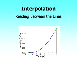
Spatial Interpolation and Extrapolation Techniques

From Point to Basin https://docs.qgis.org/2.2/en/_images/idw_interpolation.png Joseph Rungee, University of California Merced

Spatial Interpolation and Extrapolation What is interpolation and extrapolation? According to the Environmental Systems Research Institute (ESRI): Interpolation: The estimation of surface values at unsampled points based on known surface values of surrounding points. Extrapolation: Using known or observed data to infer or calculate values for unobserved times, locations or other variables outside a sampled area.

Spatial Interpolation and Extrapolation cont. These methods of spatial analysis are based on Waldo Tobler s first law of geography: Everything is related to everything else, but near things are more related than distant things. This is also known as Spatial Autocorrelation

Whats the difference? They seem very similar.. Differences: Interpolation: Calculating values between known values Less computationally intensive https://docs.qgis.org/2.2/en/_images/idw_interpolation.png

Whats the difference? Extrapolation: Calculating values beyond known values Typically requires statistical approach knowing other dependent variables http://www.xkcd.com/1281/

Why so important? It is impossible to measure every point in a space Therefore, interpolation and extrapolation are used to overcome this The information obtained, provides many benefits such as: The ability to estimate basin wide values Gives managers and decision makers better information to make more informed decisions Optimizes the use of expensive scientific equipment Minimizes natural landscape disturbance

Interpolation Methods This module will focus on two well known interpolation techniques: 1. Thiessen Polygons 2. Inverse Distance Weighted (IDW) Other popular methods 3. Kriging One of the most complex interpolators Measures the relationship between all sample points 4. Spline Utilizes curvilinear model, which allows the exceedance of sample points

Thiessen Polygons Named for American meteorologist Alfred H. Thiessen (1872-1931) Polygons generated from a set of sample points The polygons are created by drawing straight lines in between points This results in a polygon for each point for a given map extent Each polygon is given the value of the sample point within the polygon With a little geometry, a weighted value for the extent can be calculated.

Thiessen Polygon Example Step 1: Obtain extent with known sample points Let s say the points to the right are meteorological stations 1 3 2 6 4 5

Thiessen Polygon Example Step 1: Obtain extent with known sample points And values below are the station s annual precipitation values Met Station # Annual Precip (mm) 1 985 2 1015 3 963 4 1101 5 1057 6 1078

Thiessen Polygon Example Step 2: Draw straight line from point to nearest neighbor(s). Should create a map of triangles

Thiessen Polygon Example Step 3: Draw perpendicular lines in the middle of each line between points (bisectors)

Thiessen Polygon Example Step 4: Lengthen or shorten bisectors to create polygons All lines may not be used This is because it is outside of the extent But # polygons must = # points

Thiessen Polygon Example Step 5: Clean up and calculate individual areas Either Geometry or graph paper Scale at this point does not matter, only care about percentage of polygon to entire extent

Thiessen Polygon Example Step 5: Clean up and calculate individual areas 14.27% 16.13% 6.88% The red % values were calculated using graph paper and the following expression: 15.72% 27.47% %???? =# ?? ?????? ?? ???????(?) # ?? ?????? ?? ?????? 19.53% 100%

Thiessen Polygon Example Step 6: Calculate the weighted precipitation value for the area around each met station 14.27% 1 16.13% 3 6.88% 2 ??????????= ???????? ???????? ? 15.72% 27.47% 6 ???????? ?=%???? 19.53% 100% 4 5

Thiessen Polygon Example Step 7: Calculate the weighted precipitation for the entire extent ???????????= (???????? ???????? ?) Column four on table It can be seen that the weighted annual precipitation for the entire extent is 1047.2 mm Met Station # Annual Precip (mm) % Area Weighted Precip. (mm) 1 985 6.9 68.0 2 1015 16.1 163.4 3 963 14.3 137.7 4 1101 27.5 302.8 5 1057 19.5 206.1 6 1078 15.7 169.3 Sum 1047.2

Thiessen Polygon Trivia Why are the areas of the boxes irrelevant in this exercise?

Thiessen Polygon Trivia Why are the areas of the boxes irrelevant in this exercise? Because we are only concerned with the fraction of each sub-area to the entire basin, and since all boxes are the same size, units cancel! For example, if the sub-area represented by met station 1 is 20 boxes, each box is 1 square kilometers, and the area of the basin is 200 square kilometers, then: 20 1 ??2 200??2 = 0.1 or 10% Therefore, 10% of the entire basin is represented by the temperature at met station 1!

Inverse Distance Weighted (IDW) Takes auto correlation literally The nearest point to the centroid of the pixel best represents that pixel Works best for dense, evenly-spaced sample points User decides how to sample points Nearest neighbor(s) (any number) Radius around pixel centroid All sample points, etc.

Inverse Distance Weight Example Step 1: Obtain extent with known sample points Same as previous example for comparison 1 3 2 Met Station # Annual Precip (mm) 6 1 985 2 1015 4 3 963 4 1101 5 5 1057 6 1078

Inverse Distance Weight Example Step 2: Decide number of pixels We will choose six for example There will come a point where adding pixels will not longer improve the result P3 P1 P2 P6 P4 P5

Inverse Distance Weight Example Step 3: Choose which points to be included This example uses the 3 nearest neighbors P3 P1 P2 P6 P4 P5

Inverse Distance Weight Example Step 3: Choose which points to be included This example uses the 3 nearest neighbors P3 P1 P2 P6 P4 P5

Inverse Distance Weight Example Step 3: Choose which points to be included This example uses the 3 nearest neighbors P3 P1 P2 P6 P4 P5

Inverse Distance Weight Example Step 3: Choose which points to be included This example uses the 3 nearest neighbors P3 P1 P2 P6 P4 P5

Inverse Distance Weight Example Step 3: Choose which points to be included This example uses the 3 nearest neighbors P3 P1 P2 P6 P4 P5

Inverse Distance Weight Example Step 3: Choose which points to be included This example uses the 3 nearest neighbors P3 P1 P2 P6 P4 P5

Inverse Distance Weight Example Step 4: Calculate IDWs Equation: ????????????= (?? ?????????????) ?? Pixel # 1 Where ??= Met Stations Selected Distance (cm) Annual Precip (mm) Pixel Annual Precip (mm) ????????? 1 1, 2, 4 1.2, 3.8, 6.4 985, 1015, 1101 1005.8 e.g. for pixel 1 (1 1.2 985)+(1 3.8 1015)+(1 1 1.2+1 6.4 1101) = 1005.8 ?? 3.8+1 6.4

Inverse Distance Weight Example Fill out the rest! Pixel # Met Stations Selected Distance (cm) Annual Precip (mm) Pixel Annual Precip (mm) 1 1, 2, 4 1.2, 3.8, 6.4 985, 1015, 1101 1005.8 2 1, 2, 3 5.5, 2.0, 3.8 985, 1015, 963 3 2, 3, 6 6.8, 1.4, 4.5 1015, 963, 1078 4 1, 2, 4 6.3, 5.5, 1.3 985, 1015, 1101 5 2, 4, 5 5.1, 4.0, 3.4 1015, 1101, 1057 6 3, 5, 6 5.9, 3.5, 1.9 963, 1057, 1078

Inverse Distance Weight Example Step 5: Calculate weighted precip for entire basin Since the six pixels are equal size, just need to take arithmetic mean 6 1005.8+994.8+993.6+1070.3+1060.7+1052.0 = 1029.5 ?? If you remember, the Thiessen polygon basin precip was 1047.2 mm That is only a 1.7% difference between the two methods!

Issues with these two methods Spatial autocorrelation accounts for no other inputs Change in vegetation, aspect, slope, etc. Values cannot be outside the range of the sample dataset. i.e. if all samples points are forest, but trying to estimate evapotranspiration on a rock outcrop. Both these methods are also fairly subjective, and can produce relatively inconsistent results between users IDW more so than Thiessen polygons due to user defined number of pixels and method and number of choosing neighbors.

Summary Spatial interpolation and extrapolation is the process of using known values to estimate unknown values. Most spatial interpolation methods rely on spatial autocorrelation in estimating unknown values. Choosing the method of interpolation greatly depends on the user s knowledge of the known values, and how the data varies spatially. If the data varies greatly spatially, and extends beyond the range of known values, Thiessen polygons and IDW may not be the best approach.

In Class Problem Since the extent will never be a rectangle or square in the real world, let s do an example with a real basin! The watershed below is Norris River basin located primarily in northeastern Tennessee. From US EPA BASINS 4.1 (2015)

In Class Problem So let s say you want to know what the mean monthly temperature of the basin was for February 2006. Map from US EPA BASINS 4.1 (2015) Data from NOAA National Climatic Data Center

In Class Problem You select five met stations from the National Climatic Data Center (NCDC) to represent the basin with the following temperatures: Mean Monthly temp ( C) Year Month Station 2006 2006 2006 2006 2006 2 2 2 2 2 KY151080 KY154898 NC313957 TN401094 VA444180 1.76 2.64 3.52 2.68 4.21 From NOAA National Climactic Data Center Map from US EPA BASINS 4.1 (2015) Data from NOAA National Climatic Data Center

In Class Problem Using what you have learned from this lecture, draw what you think the Thiessen polygons should look like. Knowing a spatial average of temperature is beneficial in many ways, such as: Potential evapotranspiration (PET) estimation Snow-melt estimation equations Calculating components of the energy balance (i.e. latent heat) Stay on this slide until everyone has finished!

In Class Problem These polygons were generated using ArcGIS 10.3 It is alright if yours do not look exactly like this, but should be similar. Map from US EPA BASINS 4.1 (2015) Data from NOAA National Climatic Data Center

In Class Problem Calculate the percent area for each of the met stations by dividing the number of boxes in each sub area by the number of boxes in the entire basin. General expression: ??% = #?????? #?????????? 100% Map from US EPA BASINS 4.1 (2015) Data from NOAA National Climatic Data Center

In Class Problem To calculate the mean temperature of the entire basin, multiply the areal percentages with their respective mean temperature values, and then sum them all. General expression: ?????????= ?=1 ?(?????%? 100% ??) Stay on this slide until everyone is finished with their calculations!!

In Class Problem The calculations below were performed using ArcGIS 10.3 What is the difference in this weighted average vs. the arithmetic mean of the monthly temperatures? How did your answer compare? Areal percentages? Weighted Basin temp? Site Mean Monthly temp ( C) Areal percent (%) Weighted Temp ( C) Year Month Station Number 2006 2006 2006 2006 2006 2 2 2 2 2 2 1 5 3 4 KY151080 KY154898 NC313957 TN401094 VA444180 1.76 2.64 3.52 2.68 4.21 13% 27% 3% 39% 17% 0.22 0.73 0.12 1.06 0.71 2.84